6.1. Vector Data (geopandas)#
This page is a Jupyter Notebook that can be found and downloaded at the GitHub repository.
6.1.1. Introducing Geopandas#
The primary way we interact with vector data (.gpkg, .shp, .geojson, .geoparquet, etc. etc.) is via the geopandas package. This does what it sounds like - its pandas, but with additional functionality in the form of a geometry column and associated metadata that allows it to store vector geospatial information!
import geopandas as gpd

# Also we'll need matplotlib for this notebook
import matplotlib.pyplot as plt
As with everything in this documentation, GeoPandas has its own extensive documentation and examples, which you can either explore at your leisure or bit-by-bit as you need more functionality and you discover them through googling or LLMing assistance!
However, here’s a brief series of examples of how you might use it. First, we can point it to any reasonable vector file (here a .geojson), and it should be able to read it:
# Load a pre-existing map of Europe
europe_gdf = gpd.read_file('https://raw.githubusercontent.com/leakyMirror/map-of-europe/refs/heads/master/GeoJSON/europe.geojson')
Note the gdf in the variable name, which is useful shorthand to indicate you have a Geo(pandas) DataFrame. We can visualise this as with Pandas:
# Using `.head()` will limit what is shown to just the first 5 rows, useful for
# sanity checking a long dataset
europe_gdf.head()
| FID | FIPS | ISO2 | ISO3 | UN | NAME | AREA | POP2005 | REGION | SUBREGION | LON | LAT | geometry | |
|---|---|---|---|---|---|---|---|---|---|---|---|---|---|
| 0 | 0.0 | AJ | AZ | AZE | 31 | Azerbaijan | 8260 | 8352021 | 142 | 145 | 47.395 | 40.430 | MULTIPOLYGON (((45.08332 39.76804, 45.26639 39... |
| 1 | 0.0 | AL | AL | ALB | 8 | Albania | 2740 | 3153731 | 150 | 39 | 20.068 | 41.143 | POLYGON ((19.43621 41.02106, 19.45055 41.06, 1... |
| 2 | 0.0 | AM | AM | ARM | 51 | Armenia | 2820 | 3017661 | 142 | 145 | 44.563 | 40.534 | MULTIPOLYGON (((45.57305 40.63249, 45.52888 40... |
| 3 | 0.0 | BK | BA | BIH | 70 | Bosnia and Herzegovina | 5120 | 3915238 | 150 | 39 | 17.786 | 44.169 | POLYGON ((17.64984 42.88908, 17.57853 42.94382... |
| 4 | 0.0 | BU | BG | BGR | 100 | Bulgaria | 11063 | 7744591 | 150 | 151 | 25.231 | 42.761 | POLYGON ((27.87917 42.8411, 27.895 42.8025, 27... |
The most important thing is the geometry column on the far right. This is the magic geospatial data that allows us to visualise it!
europe_gdf.plot()
plt.show()
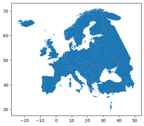
Note that just .plot() on the dataset will do a very simple matplotlib plot of the dataset. Things can get more complicated by using parameters, or by using fig, ax = plt.subplots() and ax=ax as a parameter within .plot(), we can begin to combine it with other datasets. I will do this later in the notebook.
6.1.2. Manipulating Datasets#
We have all the same functionality as pandas in terms of processing and indexing.
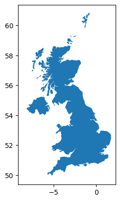
uk_gdf = europe_gdf[europe_gdf['NAME'] == 'United Kingdom']

print(f'The lat/lon boundaries of the UK are: {uk_gdf.total_bounds}.')
print(f'It has a total 2005 population of {uk_gdf['POP2005'].item()}')

uk_gdf.plot()
plt.show()
The lat/lon boundaries of the UK are: [-8.62139  49.911659  1.74944  60.844444].
It has a total 2005 population of 60244834
As you might be able to tell from the x and y axis values, we’re probably dealing with a dataset in latitude and longitude. If you have a suitable filetype that included this metadata, we can check the crs variable to make sure:
europe_gdf.crs
<Geographic 2D CRS: EPSG:4326>
Name: WGS 84
Axis Info [ellipsoidal]:
- Lat[north]: Geodetic latitude (degree)
- Lon[east]: Geodetic longitude (degree)
Area of Use:
- name: World.
- bounds: (-180.0, -90.0, 180.0, 90.0)
Datum: World Geodetic System 1984 ensemble
- Ellipsoid: WGS 84
- Prime Meridian: Greenwich
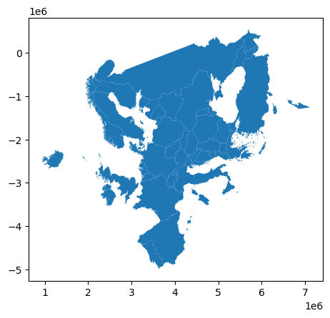
Yup! We can also convert between different CRS formats by providing the EPSG code. This is especially important if we want to start working with area/length measurements, as we want to ensure are units are in metres.
Most commonly, we will probably want to move into Polar Stereographic North (EPSG:3413) and south (EPSG:3031).
europe_gdf_polarstereographic = europe_gdf.to_crs(epsg=3413)

europe_gdf_polarstereographic.plot()
plt.show()
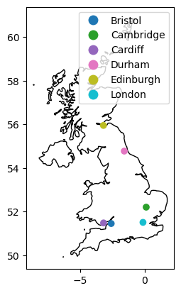
It is worth noting that GeoPandas gets its geographic geometry functionality from a base package called shapely. You can import these geometries (Point, LineString, Polygon) and create your own files if you like!
from shapely.geometry import Point

names = ["Durham", "Cambridge", "London", "Bristol", "Edinburgh", "Cardiff"]
lats = [54.7761, 52.2053, 51.5074, 51.4545, 55.9533, 51.4816]
lons = [-1.5755, 0.1218, -0.1278, -2.5879, -3.1883, -3.1791]

# Construct points list with loop
points = []
for lat, lon in zip(lats, lons):
    points.append(Point(lon, lat))  # Shapely Point expects (lon, lat)

# Create DataFrame from the lists. Columns can be presented as a dictionary
cities_df = gpd.GeoDataFrame(
    {"city": names, "lat": lats, "lon": lons},
    geometry=points,
    crs=4326
    )

fig, ax = plt.subplots()
uk_gdf.plot(ax=ax, fc='none', ec='black')  # fc: facecolor; ec: edgecolor
cities_df.plot(ax=ax, column="city", legend=True)
plt.show()
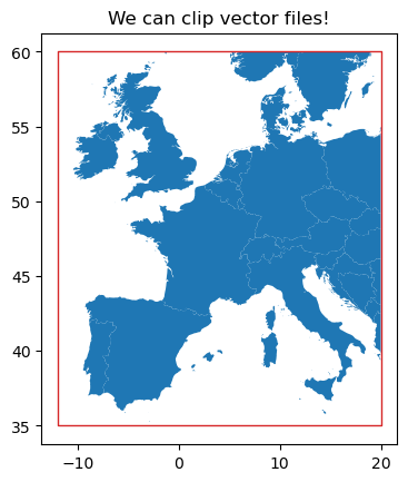
For remote sensing analysis, it is particularly useful to know the box function of shapely. This allows you to create rectangular polygons from just the bounding box (e.g. [xmin, ymin, xmax, ymax]). You can then use this for clipping datasets, including rasters!
from shapely.geometry import box

# Define shapely bbox
western_europe_bbox = box(-12, 35, 20, 60)

# Create geopandas GeoDataFrame of bbox
bbox_gdf = gpd.GeoDataFrame(geometry=[western_europe_bbox], crs=4326)

# Clip europe_gdf to bbox
western_europe_gdf = europe_gdf.clip(bbox_gdf)


fig, ax = plt.subplots()
western_europe_gdf.plot(ax=ax)
bbox_gdf.plot(ax=ax, fc='none', ec='tab:red')
ax.set_title('We can clip vector files!')
plt.show()