7. Satellite Data#
This page is a Jupyter Notebook that can be found and downloaded at the GitHub repository.
This page (and indeed, this entire section) could perhaps be considered an advanced topic. There is nothing stopping you downloading your data from a traditional GUI source (e.g. Landsat data from https://earthexplorer.usgs.gov/) and loading your datasets in using rioxarray, as explored in a previous section.
However, one of the reasons we want to learn programming is so that we can apply our analysis to very large datasets. The first aspect of this is to learn how we can download very large datasets, particularly in efficient manners. For instance, we might want to download 500 Landsat images of a glacier, but we don’t necessarily need to download 500 full Landsat scenes from EarthExplorer: perhaps we only need a specific small area, and maybe we only need a few bands. This is what interacting with data programatically aims to make efficient and easy.
7.1. Introducing STACs#
Interacting with a remote source of data normally requires something called an Application Programming Interface (API) - a little bit of software on an organsiations website that other remote programs can come and talk to (making requests and receiving a response from the API).
Many organisations have tried - and failed - to produce workable APIs for large-scale satellite data, and it was all becoming a bit of a mess. Luckily, there has been a recent consolidation around Spatio-Temporal Asset Catalogues (STACs): a standardised specification of structuring and organising geospatial data. Think of it a Dewey decimal system for geospatial data, so that no matter who is hosting the library, we know that we can walk in and the data will be organised exactly the same as in all other libraries.
As a result, we know longer need to learn how to use Python to a load of different interfaces: we only need to learn one interface (the STAC, and in particular pystac_client), and change who we are pointing to. This is a recent but rapidly growing area: I can’t promise you that everyone has a STAC, and there will be some variation (for instance, in the ice velocity and altimetry notebooks), but enough people have it that you can learn this method and download a vast range of geospatial data, including the Landsat and Sentinel (optical and radar) programmes and global DEM datasets (including ArcticDEM and REMA).
7.2. Searching for Optical Data in STACs#
7.2.1. The Microsoft Planetary Computer STAC#
Organisations with STACs include the USGS via LandsatLook, ESA/Copernicus (in progress), the Polar Geospatial Center, and OpenTopography. However, my first point of call is to consult the Microsoft Planetary Computer STAC. Here, Microsoft has hosted petabytes of data in analysis-ready formats. You can take a look at what is available to search in the catalog.
Data can be downloaded ‘anonymously’ (i.e. without registration), but download speeds may be throttled unless you can properly sign your requests. This is made easy for us through a very small additional package, unique to the MPC STAC, called planetary_computer. We can install it in the usual way, alongside the essential pystac_client whilst we’re at it:
conda install planetary-computer pystac-client
7.2.2. Connecting to a STAC#
We connect to a STAC using the pystac_client. We will need to URL link to the dynamic STAC, which will be available on various documentation. As mentioned, we use an additional magic bit of planetary_computer to facilitate our access to the MPC (other STACs will not have this):
import pystac_client
import planetary_computer  # only needed for MPC

catalog = pystac_client.Client.open(
    "https://planetarycomputer.microsoft.com/api/stac/v1",
    modifier=planetary_computer.sign_inplace,  # only needed for MPC
)
catalog
- type "Catalog"
- id "microsoft-pc"
- stac_version "1.1.0"
- description "Searchable spatiotemporal metadata describing Earth science datasets hosted by the Microsoft Planetary Computer"
links[] 135 items
0
- rel "self"
- href "https://planetarycomputer.microsoft.com/api/stac/v1"
- type "application/json"
1
- rel "root"
- href "https://planetarycomputer.microsoft.com/api/stac/v1/"
- type "application/json"
2
- rel "data"
- href "https://planetarycomputer.microsoft.com/api/stac/v1/collections"
- type "application/json"
3
- rel "conformance"
- href "https://planetarycomputer.microsoft.com/api/stac/v1/conformance"
- type "application/json"
- title "STAC/OGC conformance classes implemented by this server"
4
- rel "search"
- href "https://planetarycomputer.microsoft.com/api/stac/v1/search"
- type "application/geo+json"
- title "STAC search"
- method "GET"
5
- rel "search"
- href "https://planetarycomputer.microsoft.com/api/stac/v1/search"
- type "application/geo+json"
- title "STAC search"
- method "POST"
6
- rel "http://www.opengis.net/def/rel/ogc/1.0/queryables"
- href "https://planetarycomputer.microsoft.com/api/stac/v1/queryables"
- type "application/schema+json"
- title "Queryables"
- method "GET"
7
- rel "child"
- href "https://planetarycomputer.microsoft.com/api/stac/v1/collections/daymet-annual-pr"
- type "application/json"
- title "Daymet Annual Puerto Rico"
8
- rel "child"
- href "https://planetarycomputer.microsoft.com/api/stac/v1/collections/daymet-daily-hi"
- type "application/json"
- title "Daymet Daily Hawaii"
9
- rel "child"
- href "https://planetarycomputer.microsoft.com/api/stac/v1/collections/3dep-seamless"
- type "application/json"
- title "USGS 3DEP Seamless DEMs"
10
- rel "child"
- href "https://planetarycomputer.microsoft.com/api/stac/v1/collections/3dep-lidar-dsm"
- type "application/json"
- title "USGS 3DEP Lidar Digital Surface Model"
11
- rel "child"
- href "https://planetarycomputer.microsoft.com/api/stac/v1/collections/fia"
- type "application/json"
- title "Forest Inventory and Analysis"
12
- rel "child"
- href "https://planetarycomputer.microsoft.com/api/stac/v1/collections/gridmet"
- type "application/json"
- title "gridMET"
13
- rel "child"
- href "https://planetarycomputer.microsoft.com/api/stac/v1/collections/daymet-annual-na"
- type "application/json"
- title "Daymet Annual North America"
14
- rel "child"
- href "https://planetarycomputer.microsoft.com/api/stac/v1/collections/daymet-monthly-na"
- type "application/json"
- title "Daymet Monthly North America"
15
- rel "child"
- href "https://planetarycomputer.microsoft.com/api/stac/v1/collections/daymet-annual-hi"
- type "application/json"
- title "Daymet Annual Hawaii"
16
- rel "child"
- href "https://planetarycomputer.microsoft.com/api/stac/v1/collections/daymet-monthly-hi"
- type "application/json"
- title "Daymet Monthly Hawaii"
17
- rel "child"
- href "https://planetarycomputer.microsoft.com/api/stac/v1/collections/daymet-monthly-pr"
- type "application/json"
- title "Daymet Monthly Puerto Rico"
18
- rel "child"
- href "https://planetarycomputer.microsoft.com/api/stac/v1/collections/gnatsgo-tables"
- type "application/json"
- title "gNATSGO Soil Database - Tables"
19
- rel "child"
- href "https://planetarycomputer.microsoft.com/api/stac/v1/collections/hgb"
- type "application/json"
- title "HGB: Harmonized Global Biomass for 2010"
20
- rel "child"
- href "https://planetarycomputer.microsoft.com/api/stac/v1/collections/cop-dem-glo-30"
- type "application/json"
- title "Copernicus DEM GLO-30"
21
- rel "child"
- href "https://planetarycomputer.microsoft.com/api/stac/v1/collections/cop-dem-glo-90"
- type "application/json"
- title "Copernicus DEM GLO-90"
22
- rel "child"
- href "https://planetarycomputer.microsoft.com/api/stac/v1/collections/terraclimate"
- type "application/json"
- title "TerraClimate"
23
- rel "child"
- href "https://planetarycomputer.microsoft.com/api/stac/v1/collections/nasa-nex-gddp-cmip6"
- type "application/json"
- title "Earth Exchange Global Daily Downscaled Projections (NEX-GDDP-CMIP6)"
24
- rel "child"
- href "https://planetarycomputer.microsoft.com/api/stac/v1/collections/gpm-imerg-hhr"
- type "application/json"
- title "GPM IMERG"
25
- rel "child"
- href "https://planetarycomputer.microsoft.com/api/stac/v1/collections/gnatsgo-rasters"
- type "application/json"
- title "gNATSGO Soil Database - Rasters"
26
- rel "child"
- href "https://planetarycomputer.microsoft.com/api/stac/v1/collections/3dep-lidar-hag"
- type "application/json"
- title "USGS 3DEP Lidar Height above Ground"
27
- rel "child"
- href "https://planetarycomputer.microsoft.com/api/stac/v1/collections/io-lulc-annual-v02"
- type "application/json"
- title "10m Annual Land Use Land Cover (9-class) V2"
28
- rel "child"
- href "https://planetarycomputer.microsoft.com/api/stac/v1/collections/goes-cmi"
- type "application/json"
- title "GOES-R Cloud & Moisture Imagery"
29
- rel "child"
- href "https://planetarycomputer.microsoft.com/api/stac/v1/collections/conus404"
- type "application/json"
- title "CONUS404"
30
- rel "child"
- href "https://planetarycomputer.microsoft.com/api/stac/v1/collections/sentinel-1-rtc"
- type "application/json"
- title "Sentinel 1 Radiometrically Terrain Corrected (RTC)"
31
- rel "child"
- href "https://planetarycomputer.microsoft.com/api/stac/v1/collections/3dep-lidar-intensity"
- type "application/json"
- title "USGS 3DEP Lidar Intensity"
32
- rel "child"
- href "https://planetarycomputer.microsoft.com/api/stac/v1/collections/3dep-lidar-pointsourceid"
- type "application/json"
- title "USGS 3DEP Lidar Point Source"
33
- rel "child"
- href "https://planetarycomputer.microsoft.com/api/stac/v1/collections/mtbs"
- type "application/json"
- title "MTBS: Monitoring Trends in Burn Severity"
34
- rel "child"
- href "https://planetarycomputer.microsoft.com/api/stac/v1/collections/noaa-c-cap"
- type "application/json"
- title "C-CAP Regional Land Cover and Change"
35
- rel "child"
- href "https://planetarycomputer.microsoft.com/api/stac/v1/collections/3dep-lidar-copc"
- type "application/json"
- title "USGS 3DEP Lidar Point Cloud"
36
- rel "child"
- href "https://planetarycomputer.microsoft.com/api/stac/v1/collections/modis-64A1-061"
- type "application/json"
- title "MODIS Burned Area Monthly"
37
- rel "child"
- href "https://planetarycomputer.microsoft.com/api/stac/v1/collections/alos-fnf-mosaic"
- type "application/json"
- title "ALOS Forest/Non-Forest Annual Mosaic"
38
- rel "child"
- href "https://planetarycomputer.microsoft.com/api/stac/v1/collections/3dep-lidar-returns"
- type "application/json"
- title "USGS 3DEP Lidar Returns"
39
- rel "child"
- href "https://planetarycomputer.microsoft.com/api/stac/v1/collections/mobi"
- type "application/json"
- title "MoBI: Map of Biodiversity Importance"
40
- rel "child"
- href "https://planetarycomputer.microsoft.com/api/stac/v1/collections/landsat-c2-l2"
- type "application/json"
- title "Landsat Collection 2 Level-2"
41
- rel "child"
- href "https://planetarycomputer.microsoft.com/api/stac/v1/collections/era5-pds"
- type "application/json"
- title "ERA5 - PDS"
42
- rel "child"
- href "https://planetarycomputer.microsoft.com/api/stac/v1/collections/chloris-biomass"
- type "application/json"
- title "Chloris Biomass"
43
- rel "child"
- href "https://planetarycomputer.microsoft.com/api/stac/v1/collections/kaza-hydroforecast"
- type "application/json"
- title "HydroForecast - Kwando & Upper Zambezi Rivers"
44
- rel "child"
- href "https://planetarycomputer.microsoft.com/api/stac/v1/collections/planet-nicfi-analytic"
- type "application/json"
- title "Planet-NICFI Basemaps (Analytic)"
45
- rel "child"
- href "https://planetarycomputer.microsoft.com/api/stac/v1/collections/modis-17A2H-061"
- type "application/json"
- title "MODIS Gross Primary Productivity 8-Day"
46
- rel "child"
- href "https://planetarycomputer.microsoft.com/api/stac/v1/collections/modis-11A2-061"
- type "application/json"
- title "MODIS Land Surface Temperature/Emissivity 8-Day"
47
- rel "child"
- href "https://planetarycomputer.microsoft.com/api/stac/v1/collections/daymet-daily-pr"
- type "application/json"
- title "Daymet Daily Puerto Rico"
48
- rel "child"
- href "https://planetarycomputer.microsoft.com/api/stac/v1/collections/3dep-lidar-dtm-native"
- type "application/json"
- title "USGS 3DEP Lidar Digital Terrain Model (Native)"
49
- rel "child"
- href "https://planetarycomputer.microsoft.com/api/stac/v1/collections/3dep-lidar-classification"
- type "application/json"
- title "USGS 3DEP Lidar Classification"
50
- rel "child"
- href "https://planetarycomputer.microsoft.com/api/stac/v1/collections/3dep-lidar-dtm"
- type "application/json"
- title "USGS 3DEP Lidar Digital Terrain Model"
51
- rel "child"
- href "https://planetarycomputer.microsoft.com/api/stac/v1/collections/gap"
- type "application/json"
- title "USGS Gap Land Cover"
52
- rel "child"
- href "https://planetarycomputer.microsoft.com/api/stac/v1/collections/modis-17A2HGF-061"
- type "application/json"
- title "MODIS Gross Primary Productivity 8-Day Gap-Filled"
53
- rel "child"
- href "https://planetarycomputer.microsoft.com/api/stac/v1/collections/planet-nicfi-visual"
- type "application/json"
- title "Planet-NICFI Basemaps (Visual)"
54
- rel "child"
- href "https://planetarycomputer.microsoft.com/api/stac/v1/collections/gbif"
- type "application/json"
- title "Global Biodiversity Information Facility (GBIF)"
55
- rel "child"
- href "https://planetarycomputer.microsoft.com/api/stac/v1/collections/modis-17A3HGF-061"
- type "application/json"
- title "MODIS Net Primary Production Yearly Gap-Filled"
56
- rel "child"
- href "https://planetarycomputer.microsoft.com/api/stac/v1/collections/modis-09A1-061"
- type "application/json"
- title "MODIS Surface Reflectance 8-Day (500m)"
57
- rel "child"
- href "https://planetarycomputer.microsoft.com/api/stac/v1/collections/alos-dem"
- type "application/json"
- title "ALOS World 3D-30m"
58
- rel "child"
- href "https://planetarycomputer.microsoft.com/api/stac/v1/collections/alos-palsar-mosaic"
- type "application/json"
- title "ALOS PALSAR Annual Mosaic"
59
- rel "child"
- href "https://planetarycomputer.microsoft.com/api/stac/v1/collections/deltares-water-availability"
- type "application/json"
- title "Deltares Global Water Availability"
60
- rel "child"
- href "https://planetarycomputer.microsoft.com/api/stac/v1/collections/modis-16A3GF-061"
- type "application/json"
- title "MODIS Net Evapotranspiration Yearly Gap-Filled"
61
- rel "child"
- href "https://planetarycomputer.microsoft.com/api/stac/v1/collections/modis-21A2-061"
- type "application/json"
- title "MODIS Land Surface Temperature/3-Band Emissivity 8-Day"
62
- rel "child"
- href "https://planetarycomputer.microsoft.com/api/stac/v1/collections/us-census"
- type "application/json"
- title "US Census"
63
- rel "child"
- href "https://planetarycomputer.microsoft.com/api/stac/v1/collections/jrc-gsw"
- type "application/json"
- title "JRC Global Surface Water"
64
- rel "child"
- href "https://planetarycomputer.microsoft.com/api/stac/v1/collections/deltares-floods"
- type "application/json"
- title "Deltares Global Flood Maps"
65
- rel "child"
- href "https://planetarycomputer.microsoft.com/api/stac/v1/collections/modis-43A4-061"
- type "application/json"
- title "MODIS Nadir BRDF-Adjusted Reflectance (NBAR) Daily"
66
- rel "child"
- href "https://planetarycomputer.microsoft.com/api/stac/v1/collections/modis-09Q1-061"
- type "application/json"
- title "MODIS Surface Reflectance 8-Day (250m)"
67
- rel "child"
- href "https://planetarycomputer.microsoft.com/api/stac/v1/collections/modis-14A1-061"
- type "application/json"
- title "MODIS Thermal Anomalies/Fire Daily"
68
- rel "child"
- href "https://planetarycomputer.microsoft.com/api/stac/v1/collections/hrea"
- type "application/json"
- title "HREA: High Resolution Electricity Access"
69
- rel "child"
- href "https://planetarycomputer.microsoft.com/api/stac/v1/collections/modis-13Q1-061"
- type "application/json"
- title "MODIS Vegetation Indices 16-Day (250m)"
70
- rel "child"
- href "https://planetarycomputer.microsoft.com/api/stac/v1/collections/modis-14A2-061"
- type "application/json"
- title "MODIS Thermal Anomalies/Fire 8-Day"
71
- rel "child"
- href "https://planetarycomputer.microsoft.com/api/stac/v1/collections/sentinel-2-l2a"
- type "application/json"
- title "Sentinel-2 Level-2A"
72
- rel "child"
- href "https://planetarycomputer.microsoft.com/api/stac/v1/collections/modis-15A2H-061"
- type "application/json"
- title "MODIS Leaf Area Index/FPAR 8-Day"
73
- rel "child"
- href "https://planetarycomputer.microsoft.com/api/stac/v1/collections/modis-11A1-061"
- type "application/json"
- title "MODIS Land Surface Temperature/Emissivity Daily"
74
- rel "child"
- href "https://planetarycomputer.microsoft.com/api/stac/v1/collections/modis-15A3H-061"
- type "application/json"
- title "MODIS Leaf Area Index/FPAR 4-Day"
75
- rel "child"
- href "https://planetarycomputer.microsoft.com/api/stac/v1/collections/modis-13A1-061"
- type "application/json"
- title "MODIS Vegetation Indices 16-Day (500m)"
76
- rel "child"
- href "https://planetarycomputer.microsoft.com/api/stac/v1/collections/daymet-daily-na"
- type "application/json"
- title "Daymet Daily North America"
77
- rel "child"
- href "https://planetarycomputer.microsoft.com/api/stac/v1/collections/nrcan-landcover"
- type "application/json"
- title "Land Cover of Canada"
78
- rel "child"
- href "https://planetarycomputer.microsoft.com/api/stac/v1/collections/modis-10A2-061"
- type "application/json"
- title "MODIS Snow Cover 8-day"
79
- rel "child"
- href "https://planetarycomputer.microsoft.com/api/stac/v1/collections/ecmwf-forecast"
- type "application/json"
- title "ECMWF Open Data (real-time)"
80
- rel "child"
- href "https://planetarycomputer.microsoft.com/api/stac/v1/collections/noaa-mrms-qpe-24h-pass2"
- type "application/json"
- title "NOAA MRMS QPE 24-Hour Pass 2"
81
- rel "child"
- href "https://planetarycomputer.microsoft.com/api/stac/v1/collections/nasadem"
- type "application/json"
- title "NASADEM HGT v001"
82
- rel "child"
- href "https://planetarycomputer.microsoft.com/api/stac/v1/collections/io-lulc"
- type "application/json"
- title "Esri 10-Meter Land Cover (10-class)"
83
- rel "child"
- href "https://planetarycomputer.microsoft.com/api/stac/v1/collections/landsat-c2-l1"
- type "application/json"
- title "Landsat Collection 2 Level-1"
84
- rel "child"
- href "https://planetarycomputer.microsoft.com/api/stac/v1/collections/drcog-lulc"
- type "application/json"
- title "Denver Regional Council of Governments Land Use Land Cover"
85
- rel "child"
- href "https://planetarycomputer.microsoft.com/api/stac/v1/collections/chesapeake-lc-7"
- type "application/json"
- title "Chesapeake Land Cover (7-class)"
86
- rel "child"
- href "https://planetarycomputer.microsoft.com/api/stac/v1/collections/chesapeake-lc-13"
- type "application/json"
- title "Chesapeake Land Cover (13-class)"
87
- rel "child"
- href "https://planetarycomputer.microsoft.com/api/stac/v1/collections/chesapeake-lu"
- type "application/json"
- title "Chesapeake Land Use"
88
- rel "child"
- href "https://planetarycomputer.microsoft.com/api/stac/v1/collections/noaa-mrms-qpe-1h-pass1"
- type "application/json"
- title "NOAA MRMS QPE 1-Hour Pass 1"
89
- rel "child"
- href "https://planetarycomputer.microsoft.com/api/stac/v1/collections/noaa-mrms-qpe-1h-pass2"
- type "application/json"
- title "NOAA MRMS QPE 1-Hour Pass 2"
90
- rel "child"
- href "https://planetarycomputer.microsoft.com/api/stac/v1/collections/noaa-nclimgrid-monthly"
- type "application/json"
- title "Monthly NOAA U.S. Climate Gridded Dataset (NClimGrid)"
91
- rel "child"
- href "https://planetarycomputer.microsoft.com/api/stac/v1/collections/usda-cdl"
- type "application/json"
- title "USDA Cropland Data Layers (CDLs)"
92
- rel "child"
- href "https://planetarycomputer.microsoft.com/api/stac/v1/collections/eclipse"
- type "application/json"
- title "Urban Innovation Eclipse Sensor Data"
93
- rel "child"
- href "https://planetarycomputer.microsoft.com/api/stac/v1/collections/esa-cci-lc"
- type "application/json"
- title "ESA Climate Change Initiative Land Cover Maps (Cloud Optimized GeoTIFF)"
94
- rel "child"
- href "https://planetarycomputer.microsoft.com/api/stac/v1/collections/esa-cci-lc-netcdf"
- type "application/json"
- title "ESA Climate Change Initiative Land Cover Maps (NetCDF)"
95
- rel "child"
- href "https://planetarycomputer.microsoft.com/api/stac/v1/collections/fws-nwi"
- type "application/json"
- title "FWS National Wetlands Inventory"
96
- rel "child"
- href "https://planetarycomputer.microsoft.com/api/stac/v1/collections/usgs-lcmap-conus-v13"
- type "application/json"
- title "USGS LCMAP CONUS Collection 1.3"
97
- rel "child"
- href "https://planetarycomputer.microsoft.com/api/stac/v1/collections/usgs-lcmap-hawaii-v10"
- type "application/json"
- title "USGS LCMAP Hawaii Collection 1.0"
98
- rel "child"
- href "https://planetarycomputer.microsoft.com/api/stac/v1/collections/noaa-climate-normals-tabular"
- type "application/json"
- title "NOAA US Tabular Climate Normals"
99
- rel "child"
- href "https://planetarycomputer.microsoft.com/api/stac/v1/collections/noaa-climate-normals-netcdf"
- type "application/json"
- title "NOAA US Gridded Climate Normals (NetCDF)"
100
- rel "child"
- href "https://planetarycomputer.microsoft.com/api/stac/v1/collections/goes-glm"
- type "application/json"
- title "GOES-R Lightning Detection"
101
- rel "child"
- href "https://planetarycomputer.microsoft.com/api/stac/v1/collections/sentinel-1-grd"
- type "application/json"
- title "Sentinel 1 Level-1 Ground Range Detected (GRD)"
102
- rel "child"
- href "https://planetarycomputer.microsoft.com/api/stac/v1/collections/noaa-climate-normals-gridded"
- type "application/json"
- title "NOAA US Gridded Climate Normals (Cloud-Optimized GeoTIFF)"
103
- rel "child"
- href "https://planetarycomputer.microsoft.com/api/stac/v1/collections/aster-l1t"
- type "application/json"
- title "ASTER L1T"
104
- rel "child"
- href "https://planetarycomputer.microsoft.com/api/stac/v1/collections/cil-gdpcir-cc-by-sa"
- type "application/json"
- title "CIL Global Downscaled Projections for Climate Impacts Research (CC-BY-SA-4.0)"
105
- rel "child"
- href "https://planetarycomputer.microsoft.com/api/stac/v1/collections/naip"
- type "application/json"
- title "NAIP: National Agriculture Imagery Program"
106
- rel "child"
- href "https://planetarycomputer.microsoft.com/api/stac/v1/collections/io-lulc-9-class"
- type "application/json"
- title "10m Annual Land Use Land Cover (9-class) V1"
107
- rel "child"
- href "https://planetarycomputer.microsoft.com/api/stac/v1/collections/io-biodiversity"
- type "application/json"
- title "Biodiversity Intactness"
108
- rel "child"
- href "https://planetarycomputer.microsoft.com/api/stac/v1/collections/noaa-cdr-sea-surface-temperature-whoi"
- type "application/json"
- title "Sea Surface Temperature - WHOI CDR"
109
- rel "child"
- href "https://planetarycomputer.microsoft.com/api/stac/v1/collections/noaa-cdr-ocean-heat-content"
- type "application/json"
- title "Global Ocean Heat Content CDR"
110
- rel "child"
- href "https://planetarycomputer.microsoft.com/api/stac/v1/collections/cil-gdpcir-cc0"
- type "application/json"
- title "CIL Global Downscaled Projections for Climate Impacts Research (CC0-1.0)"
111
- rel "child"
- href "https://planetarycomputer.microsoft.com/api/stac/v1/collections/cil-gdpcir-cc-by"
- type "application/json"
- title "CIL Global Downscaled Projections for Climate Impacts Research (CC-BY-4.0)"
112
- rel "child"
- href "https://planetarycomputer.microsoft.com/api/stac/v1/collections/noaa-cdr-sea-surface-temperature-whoi-netcdf"
- type "application/json"
- title "Sea Surface Temperature - WHOI CDR NetCDFs"
113
- rel "child"
- href "https://planetarycomputer.microsoft.com/api/stac/v1/collections/noaa-cdr-sea-surface-temperature-optimum-interpolation"
- type "application/json"
- title "Sea Surface Temperature - Optimum Interpolation CDR"
114
- rel "child"
- href "https://planetarycomputer.microsoft.com/api/stac/v1/collections/modis-10A1-061"
- type "application/json"
- title "MODIS Snow Cover Daily"
115
- rel "child"
- href "https://planetarycomputer.microsoft.com/api/stac/v1/collections/sentinel-5p-l2-netcdf"
- type "application/json"
- title "Sentinel-5P Level-2"
116
- rel "child"
- href "https://planetarycomputer.microsoft.com/api/stac/v1/collections/sentinel-3-olci-wfr-l2-netcdf"
- type "application/json"
- title "Sentinel-3 Water (Full Resolution)"
117
- rel "child"
- href "https://planetarycomputer.microsoft.com/api/stac/v1/collections/noaa-cdr-ocean-heat-content-netcdf"
- type "application/json"
- title "Global Ocean Heat Content CDR NetCDFs"
118
- rel "child"
- href "https://planetarycomputer.microsoft.com/api/stac/v1/collections/hls2-l30"
- type "application/json"
- title "Harmonized Landsat Sentinel-2 (HLS) Version 2.0, Landsat Data"
119
- rel "child"
- href "https://planetarycomputer.microsoft.com/api/stac/v1/collections/sentinel-3-synergy-aod-l2-netcdf"
- type "application/json"
- title "Sentinel-3 Global Aerosol"
120
- rel "child"
- href "https://planetarycomputer.microsoft.com/api/stac/v1/collections/sentinel-3-synergy-v10-l2-netcdf"
- type "application/json"
- title "Sentinel-3 10-Day Surface Reflectance and NDVI (SPOT VEGETATION)"
121
- rel "child"
- href "https://planetarycomputer.microsoft.com/api/stac/v1/collections/sentinel-3-olci-lfr-l2-netcdf"
- type "application/json"
- title "Sentinel-3 Land (Full Resolution)"
122
- rel "child"
- href "https://planetarycomputer.microsoft.com/api/stac/v1/collections/sentinel-3-sral-lan-l2-netcdf"
- type "application/json"
- title "Sentinel-3 Land Radar Altimetry"
123
- rel "child"
- href "https://planetarycomputer.microsoft.com/api/stac/v1/collections/sentinel-3-slstr-lst-l2-netcdf"
- type "application/json"
- title "Sentinel-3 Land Surface Temperature"
124
- rel "child"
- href "https://planetarycomputer.microsoft.com/api/stac/v1/collections/sentinel-3-slstr-wst-l2-netcdf"
- type "application/json"
- title "Sentinel-3 Sea Surface Temperature"
125
- rel "child"
- href "https://planetarycomputer.microsoft.com/api/stac/v1/collections/sentinel-3-sral-wat-l2-netcdf"
- type "application/json"
- title "Sentinel-3 Ocean Radar Altimetry"
126
- rel "child"
- href "https://planetarycomputer.microsoft.com/api/stac/v1/collections/hls2-s30"
- type "application/json"
- title "Harmonized Landsat Sentinel-2 (HLS) Version 2.0, Sentinel-2 Data"
127
- rel "child"
- href "https://planetarycomputer.microsoft.com/api/stac/v1/collections/ms-buildings"
- type "application/json"
- title "Microsoft Building Footprints"
128
- rel "child"
- href "https://planetarycomputer.microsoft.com/api/stac/v1/collections/sentinel-3-slstr-frp-l2-netcdf"
- type "application/json"
- title "Sentinel-3 Fire Radiative Power"
129
- rel "child"
- href "https://planetarycomputer.microsoft.com/api/stac/v1/collections/sentinel-3-synergy-syn-l2-netcdf"
- type "application/json"
- title "Sentinel-3 Land Surface Reflectance and Aerosol"
130
- rel "child"
- href "https://planetarycomputer.microsoft.com/api/stac/v1/collections/sentinel-3-synergy-vgp-l2-netcdf"
- type "application/json"
- title "Sentinel-3 Top of Atmosphere Reflectance (SPOT VEGETATION)"
131
- rel "child"
- href "https://planetarycomputer.microsoft.com/api/stac/v1/collections/sentinel-3-synergy-vg1-l2-netcdf"
- type "application/json"
- title "Sentinel-3 1-Day Surface Reflectance and NDVI (SPOT VEGETATION)"
132
- rel "child"
- href "https://planetarycomputer.microsoft.com/api/stac/v1/collections/esa-worldcover"
- type "application/json"
- title "ESA WorldCover"
133
- rel "service-desc"
- href "https://planetarycomputer.microsoft.com/api/stac/v1/openapi.json"
- type "application/vnd.oai.openapi+json;version=3.0"
- title "OpenAPI service description"
134
- rel "service-doc"
- href "https://planetarycomputer.microsoft.com/api/stac/v1/docs"
- type "text/html"
- title "OpenAPI service documentation"
conformsTo[] 15 items
- 0 "http://www.opengis.net/spec/cql2/1.0/conf/cql2-json"
- 1 "https://api.stacspec.org/v1.0.0/core"
- 2 "http://www.opengis.net/spec/ogcapi-features-1/1.0/conf/oas30"
- 3 "https://api.stacspec.org/v1.0.0-rc.2/item-search#filter"
- 4 "https://api.stacspec.org/v1.0.0/item-search#query"
- 5 "http://www.opengis.net/spec/ogcapi-features-3/1.0/conf/filter"
- 6 "https://api.stacspec.org/v1.0.0/item-search#sort"
- 7 "https://api.stacspec.org/v1.0.0/collections"
- 8 "http://www.opengis.net/spec/ogcapi-features-1/1.0/conf/geojson"
- 9 "https://api.stacspec.org/v1.0.0/item-search"
- 10 "http://www.opengis.net/spec/cql2/1.0/conf/basic-cql2"
- 11 "http://www.opengis.net/spec/cql2/1.0/conf/cql2-text"
- 12 "http://www.opengis.net/spec/ogcapi-features-1/1.0/conf/core"
- 13 "https://api.stacspec.org/v1.0.0/ogcapi-features"
- 14 "https://api.stacspec.org/v1.0.0/item-search#fields"
- title "Microsoft Planetary Computer STAC API"
It’s challenging to understand what’s going on with this returned object, but at least we know we’ve succesfully connected.
Now, we can search individual collections. We can see all the collections in the MPC catalogue, and individual collections will show us more data. For instance, at the Landsat Collection-2 Level-2 site, we can see that the collection name is landsat-c2-l2, as well as the various “assets” contained within the dataset, such as all the bands and metadata.
We can assess the collection by getting it as a variable:
collection = catalog.get_collection("landsat-c2-l2")
collection
- type "Collection"
- id "landsat-c2-l2"
- stac_version "1.1.0"
- description "Landsat Collection 2 Level-2 [Science Products](https://www.usgs.gov/landsat-missions/landsat-collection-2-level-2-science-products), consisting of atmospherically corrected [surface reflectance](https://www.usgs.gov/landsat-missions/landsat-collection-2-surface-reflectance) and [surface temperature](https://www.usgs.gov/landsat-missions/landsat-collection-2-surface-temperature) image data. Collection 2 Level-2 Science Products are available from August 22, 1982 to present. This dataset represents the global archive of Level-2 data from [Landsat Collection 2](https://www.usgs.gov/core-science-systems/nli/landsat/landsat-collection-2) acquired by the [Thematic Mapper](https://landsat.gsfc.nasa.gov/thematic-mapper/) onboard Landsat 4 and 5, the [Enhanced Thematic Mapper](https://landsat.gsfc.nasa.gov/the-enhanced-thematic-mapper-plus-etm/) onboard Landsat 7, and the [Operatational Land Imager](https://landsat.gsfc.nasa.gov/satellites/landsat-8/spacecraft-instruments/operational-land-imager/) and [Thermal Infrared Sensor](https://landsat.gsfc.nasa.gov/satellites/landsat-8/spacecraft-instruments/thermal-infrared-sensor/) onboard Landsat 8 and 9. Images are stored in [cloud-optimized GeoTIFF](https://www.cogeo.org/) format. "
links[] 9 items
0
- rel "items"
- href "https://planetarycomputer.microsoft.com/api/stac/v1/collections/landsat-c2-l2/items"
- type "application/geo+json"
1
- rel "parent"
- href "https://planetarycomputer.microsoft.com/api/stac/v1/"
- type "application/json"
2
- rel "root"
- href "https://planetarycomputer.microsoft.com/api/stac/v1"
- type "application/json"
- title "Microsoft Planetary Computer STAC API"
3
- rel "self"
- href "https://planetarycomputer.microsoft.com/api/stac/v1/collections/landsat-c2-l2"
- type "application/json"
4
- rel "cite-as"
- href "https://doi.org/10.5066/P9IAXOVV"
- title "Landsat 4-5 TM Collection 2 Level-2"
5
- rel "cite-as"
- href "https://doi.org/10.5066/P9C7I13B"
- title "Landsat 7 ETM+ Collection 2 Level-2"
6
- rel "cite-as"
- href "https://doi.org/10.5066/P9OGBGM6"
- title "Landsat 8-9 OLI/TIRS Collection 2 Level-2"
7
- rel "license"
- href "https://www.usgs.gov/core-science-systems/hdds/data-policy"
- title "Public Domain"
8
- rel "describedby"
- href "https://planetarycomputer.microsoft.com/dataset/landsat-c2-l2"
- type "text/html"
- title "Human readable dataset overview and reference"
stac_extensions[] 6 items
- 0 "https://stac-extensions.github.io/item-assets/v1.0.0/schema.json"
- 1 "https://stac-extensions.github.io/view/v1.0.0/schema.json"
- 2 "https://stac-extensions.github.io/scientific/v1.0.0/schema.json"
- 3 "https://stac-extensions.github.io/raster/v1.0.0/schema.json"
- 4 "https://stac-extensions.github.io/eo/v1.0.0/schema.json"
- 5 "https://stac-extensions.github.io/table/v1.2.0/schema.json"
item_assets
qa
- type "image/tiff; application=geotiff; profile=cloud-optimized"
roles[] 1 items
- 0 "data"
- title "Surface Temperature Quality Assessment Band"
- description "Collection 2 Level-2 Quality Assessment Band (ST_QA) Surface Temperature Product"
raster:bands[] 1 items
0
- unit "kelvin"
- scale 0.01
- nodata -9999
- data_type "int16"
- spatial_resolution 30
ang
- type "text/plain"
roles[] 1 items
- 0 "metadata"
- title "Angle Coefficients File"
- description "Collection 2 Level-1 Angle Coefficients File"
red
- type "image/tiff; application=geotiff; profile=cloud-optimized"
roles[] 2 items
- 0 "data"
- 1 "reflectance"
- title "Red Band"
eo:bands[] 1 items
0
- common_name "red"
- description "Visible red"
raster:bands[] 1 items
0
- scale 2.75e-05
- nodata 0
- offset -0.2
- data_type "uint16"
- spatial_resolution 30
blue
- type "image/tiff; application=geotiff; profile=cloud-optimized"
roles[] 2 items
- 0 "data"
- 1 "reflectance"
- title "Blue Band"
eo:bands[] 1 items
0
- common_name "blue"
- description "Visible blue"
raster:bands[] 1 items
0
- scale 2.75e-05
- nodata 0
- offset -0.2
- data_type "uint16"
- spatial_resolution 30
drad
- type "image/tiff; application=geotiff; profile=cloud-optimized"
roles[] 1 items
- 0 "data"
- title "Downwelled Radiance Band"
- description "Collection 2 Level-2 Downwelled Radiance Band (ST_DRAD) Surface Temperature Product"
raster:bands[] 1 items
0
- unit "watt/steradian/square_meter/micrometer"
- scale 0.001
- nodata -9999
- data_type "int16"
- spatial_resolution 30
emis
- type "image/tiff; application=geotiff; profile=cloud-optimized"
roles[] 1 items
- 0 "data"
- title "Emissivity Band"
- description "Collection 2 Level-2 Emissivity Band (ST_EMIS) Surface Temperature Product"
raster:bands[] 1 items
0
- unit "emissivity coefficient"
- scale 0.0001
- nodata -9999
- data_type "int16"
- spatial_resolution 30
emsd
- type "image/tiff; application=geotiff; profile=cloud-optimized"
roles[] 1 items
- 0 "data"
- title "Emissivity Standard Deviation Band"
- description "Collection 2 Level-2 Emissivity Standard Deviation Band (ST_EMSD) Surface Temperature Product"
raster:bands[] 1 items
0
- unit "emissivity coefficient"
- scale 0.0001
- nodata -9999
- data_type "int16"
- spatial_resolution 30
lwir
- type "image/tiff; application=geotiff; profile=cloud-optimized"
roles[] 2 items
- 0 "data"
- 1 "temperature"
- title "Surface Temperature Band"
eo:bands[] 1 items
0
- common_name "lwir"
- description "Long-wave infrared"
- description "Collection 2 Level-2 Thermal Infrared Band (ST_B6) Surface Temperature"
raster:bands[] 1 items
0
- unit "kelvin"
- scale 0.00341802
- nodata 0
- offset 149.0
- data_type "uint16"
- spatial_resolution 30
trad
- type "image/tiff; application=geotiff; profile=cloud-optimized"
roles[] 1 items
- 0 "data"
- title "Thermal Radiance Band"
- description "Collection 2 Level-2 Thermal Radiance Band (ST_TRAD) Surface Temperature Product"
raster:bands[] 1 items
0
- unit "watt/steradian/square_meter/micrometer"
- scale 0.001
- nodata -9999
- data_type "int16"
- spatial_resolution 30
urad
- type "image/tiff; application=geotiff; profile=cloud-optimized"
roles[] 1 items
- 0 "data"
- title "Upwelled Radiance Band"
- description "Collection 2 Level-2 Upwelled Radiance Band (ST_URAD) Surface Temperature Product"
raster:bands[] 1 items
0
- unit "watt/steradian/square_meter/micrometer"
- scale 0.001
- nodata -9999
- data_type "int16"
- spatial_resolution 30
atran
- type "image/tiff; application=geotiff; profile=cloud-optimized"
roles[] 1 items
- 0 "data"
- title "Atmospheric Transmittance Band"
- description "Collection 2 Level-2 Atmospheric Transmittance Band (ST_ATRAN) Surface Temperature Product"
raster:bands[] 1 items
0
- scale 0.0001
- nodata -9999
- data_type "int16"
- spatial_resolution 30
cdist
- type "image/tiff; application=geotiff; profile=cloud-optimized"
roles[] 1 items
- 0 "data"
- title "Cloud Distance Band"
- description "Collection 2 Level-2 Cloud Distance Band (ST_CDIST) Surface Temperature Product"
raster:bands[] 1 items
0
- unit "kilometer"
- scale 0.01
- nodata -9999
- data_type "int16"
- spatial_resolution 30
green
- type "image/tiff; application=geotiff; profile=cloud-optimized"
roles[] 2 items
- 0 "data"
- 1 "reflectance"
- title "Green Band"
eo:bands[] 1 items
0
- common_name "green"
- description "Visible green"
- center_wavelength 0.56
raster:bands[] 1 items
0
- scale 2.75e-05
- nodata 0
- offset -0.2
- data_type "uint16"
- spatial_resolution 30
nir08
- type "image/tiff; application=geotiff; profile=cloud-optimized"
roles[] 2 items
- 0 "data"
- 1 "reflectance"
- title "Near Infrared Band 0.8"
eo:bands[] 1 items
0
- common_name "nir08"
- description "Near infrared"
raster:bands[] 1 items
0
- scale 2.75e-05
- nodata 0
- offset -0.2
- data_type "uint16"
- spatial_resolution 30
lwir11
- gsd 100
- type "image/tiff; application=geotiff; profile=cloud-optimized"
roles[] 2 items
- 0 "data"
- 1 "temperature"
- title "Surface Temperature Band"
eo:bands[] 1 items
0
- name "TIRS_B10"
- common_name "lwir11"
- description "Long-wave infrared"
- center_wavelength 10.9
- full_width_half_max 0.59
- description "Collection 2 Level-2 Thermal Infrared Band (ST_B10) Surface Temperature"
raster:bands[] 1 items
0
- unit "kelvin"
- scale 0.00341802
- nodata 0
- offset 149.0
- data_type "uint16"
- spatial_resolution 30
swir16
- type "image/tiff; application=geotiff; profile=cloud-optimized"
roles[] 2 items
- 0 "data"
- 1 "reflectance"
- title "Short-wave Infrared Band 1.6"
eo:bands[] 1 items
0
- common_name "swir16"
- description "Short-wave infrared"
raster:bands[] 1 items
0
- scale 2.75e-05
- nodata 0
- offset -0.2
- data_type "uint16"
- spatial_resolution 30
swir22
- type "image/tiff; application=geotiff; profile=cloud-optimized"
roles[] 2 items
- 0 "data"
- 1 "reflectance"
- title "Short-wave Infrared Band 2.2"
eo:bands[] 1 items
0
- common_name "swir22"
- description "Short-wave infrared"
- description "Collection 2 Level-2 Short-wave Infrared Band 2.2 (SR_B7) Surface Reflectance"
raster:bands[] 1 items
0
- scale 2.75e-05
- nodata 0
- offset -0.2
- data_type "uint16"
- spatial_resolution 30
coastal
- type "image/tiff; application=geotiff; profile=cloud-optimized"
roles[] 2 items
- 0 "data"
- 1 "reflectance"
- title "Coastal/Aerosol Band"
eo:bands[] 1 items
0
- name "OLI_B1"
- common_name "coastal"
- description "Coastal/Aerosol"
- center_wavelength 0.44
- full_width_half_max 0.02
- description "Collection 2 Level-2 Coastal/Aerosol Band (SR_B1) Surface Reflectance"
raster:bands[] 1 items
0
- scale 2.75e-05
- nodata 0
- offset -0.2
- data_type "uint16"
- spatial_resolution 30
mtl.txt
- type "text/plain"
roles[] 1 items
- 0 "metadata"
- title "Product Metadata File (txt)"
- description "Collection 2 Level-2 Product Metadata File (txt)"
mtl.xml
- type "application/xml"
roles[] 1 items
- 0 "metadata"
- title "Product Metadata File (xml)"
- description "Collection 2 Level-2 Product Metadata File (xml)"
cloud_qa
- type "image/tiff; application=geotiff; profile=cloud-optimized"
roles[] 4 items
- 0 "cloud"
- 1 "cloud-shadow"
- 2 "snow-ice"
- 3 "water-mask"
- title "Cloud Quality Assessment Band"
- description "Collection 2 Level-2 Cloud Quality Assessment Band (SR_CLOUD_QA) Surface Reflectance Product"
raster:bands[] 1 items
0
- unit "bit index"
- data_type "uint8"
- spatial_resolution 30
classification:bitfields[] 6 items
0
- name "ddv"
- length 1
- offset 0
classes[] 2 items
0
- name "not_ddv"
- value 0
- description "Pixel has no DDV"
1
- name "ddv"
- value 1
- description "Pixel has DDV"
- description "Dense Dark Vegetation (DDV)"
1
- name "cloud"
- length 1
- offset 1
classes[] 2 items
0
- name "not_cloud"
- value 0
- description "Pixel has no cloud"
1
- name "cloud"
- value 1
- description "Pixel has cloud"
- description "Cloud mask"
2
- name "cloud_shadow"
- length 1
- offset 2
classes[] 2 items
0
- name "not_shadow"
- value 0
- description "Pixel has no cloud shadow"
1
- name "shadow"
- value 1
- description "Pixel has cloud shadow"
- description "Cloud shadow mask"
3
- name "cloud_adjacent"
- length 1
- offset 3
classes[] 2 items
0
- name "not_adjacent"
- value 0
- description "Pixel is not adjacent to cloud"
1
- name "adjacent"
- value 1
- description "Pixel is adjacent to cloud"
- description "Cloud adjacency"
4
- name "snow"
- length 1
- offset 4
classes[] 2 items
0
- name "not_snow"
- value 0
- description "Pixel is not snow"
1
- name "shadow"
- value 1
- description "Pixel is snow"
- description "Snow mask"
5
- name "water"
- length 1
- offset 5
classes[] 2 items
0
- name "not_water"
- value 0
- description "Pixel is not water"
1
- name "water"
- value 1
- description "Pixel is water"
- description "Water mask"
mtl.json
- type "application/json"
roles[] 1 items
- 0 "metadata"
- title "Product Metadata File (json)"
- description "Collection 2 Level-2 Product Metadata File (json)"
qa_pixel
- type "image/tiff; application=geotiff; profile=cloud-optimized"
roles[] 4 items
- 0 "cloud"
- 1 "cloud-shadow"
- 2 "snow-ice"
- 3 "water-mask"
- title "Pixel Quality Assessment Band"
- description "Collection 2 Level-1 Pixel Quality Assessment Band (QA_PIXEL)"
raster:bands[] 1 items
0
- unit "bit index"
- nodata 1
- data_type "uint16"
- spatial_resolution 30
qa_radsat
- type "image/tiff; application=geotiff; profile=cloud-optimized"
roles[] 1 items
- 0 "saturation"
raster:bands[] 1 items
0
- unit "bit index"
- data_type "uint16"
- spatial_resolution 30
qa_aerosol
- type "image/tiff; application=geotiff; profile=cloud-optimized"
roles[] 2 items
- 0 "data-mask"
- 1 "water-mask"
- title "Aerosol Quality Assessment Band"
- description "Collection 2 Level-2 Aerosol Quality Assessment Band (SR_QA_AEROSOL) Surface Reflectance Product"
raster:bands[] 1 items
0
- unit "bit index"
- nodata 1
- data_type "uint8"
- spatial_resolution 30
classification:bitfields[] 5 items
0
- name "fill"
- length 1
- offset 0
classes[] 2 items
0
- name "not_fill"
- value 0
- description "Pixel is not fill"
1
- name "fill"
- value 1
- description "Pixel is fill"
- description "Image or fill data"
1
- name "retrieval"
- length 1
- offset 1
classes[] 2 items
0
- name "not_valid"
- value 0
- description "Pixel retrieval is not valid"
1
- name "valid"
- value 1
- description "Pixel retrieval is valid"
- description "Valid aerosol retrieval"
2
- name "water"
- length 1
- offset 2
classes[] 2 items
0
- name "not_water"
- value 0
- description "Pixel is not water"
1
- name "water"
- value 1
- description "Pixel is water"
- description "Water mask"
3
- name "interpolated"
- length 1
- offset 5
classes[] 2 items
0
- name "not_interpolated"
- value 0
- description "Pixel is not interpolated aerosol"
1
- name "interpolated"
- value 1
- description "Pixel is interpolated aerosol"
- description "Aerosol interpolation"
4
- name "level"
- length 2
- offset 6
classes[] 4 items
0
- name "climatology"
- value 0
- description "No aerosol correction applied"
1
- name "low"
- value 1
- description "Low aerosol level"
2
- name "medium"
- value 2
- description "Medium aerosol level"
3
- name "high"
- value 3
- description "High aerosol level"
- description "Aerosol level"
atmos_opacity
- type "image/tiff; application=geotiff; profile=cloud-optimized"
roles[] 1 items
- 0 "data"
- title "Atmospheric Opacity Band"
- description "Collection 2 Level-2 Atmospheric Opacity Band (SR_ATMOS_OPACITY) Surface Reflectance Product"
raster:bands[] 1 items
0
- scale 0.001
- nodata -9999
- data_type "int16"
- spatial_resolution 30
- msft:group_id "landsat"
- msft:container "landsat-c2"
- msft:storage_account "landsateuwest"
- msft:short_description "Landsat Collection 2 Level-2 data from the Thematic Mapper (TM) onboard Landsat 4 and 5, the Enhanced Thematic Mapper Plus (ETM+) onboard Landsat 7, and the Operational Land Imager (OLI) and Thermal Infrared Sensor (TIRS) onboard Landsat 8 and 9."
- msft:region "westeurope"
- title "Landsat Collection 2 Level-2"
extent
spatial
bbox[] 1 items
0[] 4 items
- 0 -180.0
- 1 -90.0
- 2 180.0
- 3 90.0
temporal
interval[] 1 items
0[] 2 items
- 0 "1982-08-22T00:00:00Z"
- 1 None
- license "proprietary"
keywords[] 8 items
- 0 "Landsat"
- 1 "USGS"
- 2 "NASA"
- 3 "Satellite"
- 4 "Global"
- 5 "Imagery"
- 6 "Reflectance"
- 7 "Temperature"
providers[] 3 items
0
- name "NASA"
roles[] 2 items
- 0 "producer"
- 1 "licensor"
- url "https://landsat.gsfc.nasa.gov/"
1
- name "USGS"
roles[] 3 items
- 0 "producer"
- 1 "processor"
- 2 "licensor"
- url "https://www.usgs.gov/landsat-missions/landsat-collection-2-level-2-science-products"
2
- name "Microsoft"
roles[] 1 items
- 0 "host"
- url "https://planetarycomputer.microsoft.com"
summaries
gsd[] 4 items
- 0 30
- 1 60
- 2 100
- 3 120
sci:doi[] 3 items
- 0 "10.5066/P9IAXOVV"
- 1 "10.5066/P9C7I13B"
- 2 "10.5066/P9OGBGM6"
eo:bands[] 22 items
0
- name "TM_B1"
- common_name "blue"
- description "Visible blue (Thematic Mapper)"
- center_wavelength 0.49
- full_width_half_max 0.07
1
- name "TM_B2"
- common_name "green"
- description "Visible green (Thematic Mapper)"
- center_wavelength 0.56
- full_width_half_max 0.08
2
- name "TM_B3"
- common_name "red"
- description "Visible red (Thematic Mapper)"
- center_wavelength 0.66
- full_width_half_max 0.06
3
- name "TM_B4"
- common_name "nir08"
- description "Near infrared (Thematic Mapper)"
- center_wavelength 0.83
- full_width_half_max 0.14
4
- name "TM_B5"
- common_name "swir16"
- description "Short-wave infrared (Thematic Mapper)"
- center_wavelength 1.65
- full_width_half_max 0.2
5
- name "TM_B6"
- common_name "lwir"
- description "Long-wave infrared (Thematic Mapper)"
- center_wavelength 11.45
- full_width_half_max 2.1
6
- name "TM_B7"
- common_name "swir22"
- description "Short-wave infrared (Thematic Mapper)"
- center_wavelength 2.22
- full_width_half_max 0.27
7
- name "ETM_B1"
- common_name "blue"
- description "Visible blue (Enhanced Thematic Mapper Plus)"
- center_wavelength 0.48
- full_width_half_max 0.07
8
- name "ETM_B2"
- common_name "green"
- description "Visible green (Enhanced Thematic Mapper Plus)"
- center_wavelength 0.56
- full_width_half_max 0.08
9
- name "ETM_B3"
- common_name "red"
- description "Visible red (Enhanced Thematic Mapper Plus)"
- center_wavelength 0.66
- full_width_half_max 0.06
10
- name "ETM_B4"
- common_name "nir08"
- description "Near infrared (Enhanced Thematic Mapper Plus)"
- center_wavelength 0.84
- full_width_half_max 0.13
11
- name "ETM_B5"
- common_name "swir16"
- description "Short-wave infrared (Enhanced Thematic Mapper Plus)"
- center_wavelength 1.65
- full_width_half_max 0.2
12
- name "ETM_B6"
- common_name "lwir"
- description "Long-wave infrared (Enhanced Thematic Mapper Plus)"
- center_wavelength 11.34
- full_width_half_max 2.05
13
- name "ETM_B7"
- common_name "swir22"
- description "Short-wave infrared (Enhanced Thematic Mapper Plus)"
- center_wavelength 2.2
- full_width_half_max 0.28
14
- name "OLI_B1"
- common_name "coastal"
- description "Coastal/Aerosol (Operational Land Imager)"
- center_wavelength 0.44
- full_width_half_max 0.02
15
- name "OLI_B2"
- common_name "blue"
- description "Visible blue (Operational Land Imager)"
- center_wavelength 0.48
- full_width_half_max 0.06
16
- name "OLI_B3"
- common_name "green"
- description "Visible green (Operational Land Imager)"
- center_wavelength 0.56
- full_width_half_max 0.06
17
- name "OLI_B4"
- common_name "red"
- description "Visible red (Operational Land Imager)"
- center_wavelength 0.65
- full_width_half_max 0.04
18
- name "OLI_B5"
- common_name "nir08"
- description "Near infrared (Operational Land Imager)"
- center_wavelength 0.87
- full_width_half_max 0.03
19
- name "OLI_B6"
- common_name "swir16"
- description "Short-wave infrared (Operational Land Imager)"
- center_wavelength 1.61
- full_width_half_max 0.09
20
- name "OLI_B7"
- common_name "swir22"
- description "Short-wave infrared (Operational Land Imager)"
- center_wavelength 2.2
- full_width_half_max 0.19
21
- name "TIRS_B10"
- common_name "lwir11"
- description "Long-wave infrared (Thermal Infrared Sensor)"
- center_wavelength 10.9
- full_width_half_max 0.59
platform[] 5 items
- 0 "landsat-4"
- 1 "landsat-5"
- 2 "landsat-7"
- 3 "landsat-8"
- 4 "landsat-9"
instruments[] 4 items
- 0 "tm"
- 1 "etm+"
- 2 "oli"
- 3 "tirs"
view:off_nadir
- minimum 0
- maximum 15
assets
thumbnail
- href "https://ai4edatasetspublicassets.blob.core.windows.net/assets/pc_thumbnails/landsat-c2-l2-thumb.png"
- type "image/png"
- title "Landsat Collection 2 Level-2 thumbnail"
roles[] 1 items
- 0 "thumbnail"
geoparquet-items
- href "abfs://items/landsat-c2-l2.parquet"
- type "application/x-parquet"
- title "GeoParquet STAC items"
- description "Snapshot of the collection's STAC items exported to GeoParquet format."
msft:partition_info
- is_partitioned True
- partition_frequency "MS"
table:storage_options
- account_name "pcstacitems"
- credential "st=2025-09-23T13%3A52%3A19Z&se=2025-09-24T14%3A37%3A19Z&sp=rl&sv=2025-07-05&sr=c&skoid=9c8ff44a-6a2c-4dfb-b298-1c9212f64d9a&sktid=72f988bf-86f1-41af-91ab-2d7cd011db47&skt=2025-09-23T22%3A33%3A25Z&ske=2025-09-30T22%3A33%3A25Z&sks=b&skv=2025-07-05&sig=1H6t5jjKuxK3%2BbquOU5r6WCYfC5%2Br57NmDF0SgyhHNw%3D"
roles[] 1 items
- 0 "stac-items"
Particularly useful submenues here are the item_assets and summaries tabs, where you can see what bands are available.
7.2.3. Searching a STAC#
We can search the catalogue using a standardised search tool. There are always some consistent things you can search a STAC catalogue for, including time_range and some sort of spatial search - which could be bbox in the form of [xmin, ymin, xmax, ymax], or using the intersects parameter by feeding a GeoJSON or shapely geometry feature. All will work in lat/lon only, as this is how STACs are spatially indexed.
Let’s search for coverage of Helheim. We will ultimately want to work in Polar Stereographic North, so we will begin with a bounding box in this format and convert to a WGS84 lat/lon version.
import geopandas as gpd
from shapely.geometry import box

issunguata_bounds_3413 = -235000,-2497000,-217000,-2489000

issunguata_gdf_3413 = gpd.GeoDataFrame(geometry=[box(*issunguata_bounds_3413)], crs="epsg:3413")
issunguata_gdf_4326 = issunguata_gdf_3413.to_crs(4326)

issunguata_bounds_4326 = issunguata_gdf_4326.geometry.values[0].bounds

# Get EPSG:4326 geometry for feeding in to STAC search
issunguata_4326_geom = issunguata_gdf_4326.geometry.values[0]
Now let’s get a search set up.
collection = "landsat-c2-l2"
time_range = "2024-05-01/2024-09-01"
geom = issunguata_4326_geom

search = catalog.search(
    collections=[collection],
    intersects=geom,
    datetime=time_range,
)

# Check how many items were returned
items = search.item_collection()
print(f"Query returns {len(items)} Items")
Query returns 74 Items
23 valid items have been returned. Let’s take a look at what the first result looks like:
item = items[0]
item
- type "Feature"
- stac_version "1.1.0"
stac_extensions[] 7 items
- 0 "https://stac-extensions.github.io/raster/v1.1.0/schema.json"
- 1 "https://stac-extensions.github.io/eo/v1.1.0/schema.json"
- 2 "https://stac-extensions.github.io/view/v1.0.0/schema.json"
- 3 "https://stac-extensions.github.io/projection/v2.0.0/schema.json"
- 4 "https://landsat.usgs.gov/stac/landsat-extension/v1.1.1/schema.json"
- 5 "https://stac-extensions.github.io/classification/v2.0.0/schema.json"
- 6 "https://stac-extensions.github.io/scientific/v1.0.0/schema.json"
- id "LC09_L2SP_008013_20240901_02_T2"
geometry
- type "Polygon"
coordinates[] 1 items
0[] 5 items
0[] 2 items
- 0 -52.19759414850223
- 1 68.06365228705155
1[] 2 items
- 0 -53.80723554356294
- 1 66.43055656508004
2[] 2 items
- 0 -49.944305830315265
- 1 65.79597525178143
3[] 2 items
- 0 -48.107148976219634
- 1 67.39570468981069
4[] 2 items
- 0 -52.19759414850223
- 1 68.06365228705155
bbox[] 4 items
- 0 -54.062647468839806
- 1 65.76530564353911
- 2 -47.98280040644627
- 3 68.0509243564609
properties
- gsd 30
- created "2024-10-05T09:21:19.459948Z"
- sci:doi "10.5066/P9OGBGM6"
- datetime "2024-09-01T14:54:58.857174Z"
- platform "landsat-9"
proj:shape[] 2 items
- 0 8501
- 1 8451
- description "Landsat Collection 2 Level-2"
instruments[] 2 items
- 0 "oli"
- 1 "tirs"
- eo:cloud_cover 100.0
proj:transform[] 6 items
- 0 30.0
- 1 0.0
- 2 372285.0
- 3 0.0
- 4 -30.0
- 5 7551615.0
- view:off_nadir 0
- landsat:wrs_row "013"
- landsat:scene_id "LC90080132024245LGN00"
- landsat:wrs_path "008"
- landsat:wrs_type "2"
- view:sun_azimuth 171.66797215
- landsat:correction "L2SP"
- view:sun_elevation 30.80181717
- landsat:cloud_cover_land 100.0
- landsat:collection_number "02"
- landsat:collection_category "T2"
- proj:code "EPSG:32622"
links[] 8 items
0
- rel "collection"
- href "https://planetarycomputer.microsoft.com/api/stac/v1/collections/landsat-c2-l2"
- type "application/json"
1
- rel "parent"
- href "https://planetarycomputer.microsoft.com/api/stac/v1/collections/landsat-c2-l2"
- type "application/json"
2
- rel "root"
- href "https://planetarycomputer.microsoft.com/api/stac/v1"
- type "application/json"
- title "Microsoft Planetary Computer STAC API"
3
- rel "self"
- href "https://planetarycomputer.microsoft.com/api/stac/v1/collections/landsat-c2-l2/items/LC09_L2SP_008013_20240901_02_T2"
- type "application/geo+json"
4
- rel "cite-as"
- href "https://doi.org/10.5066/P9OGBGM6"
- title "Landsat 8-9 OLI/TIRS Collection 2 Level-2"
5
- rel "via"
- href "https://landsatlook.usgs.gov/stac-server/collections/landsat-c2l2-sr/items/LC09_L2SP_008013_20240901_20240903_02_T2_SR"
- type "application/json"
- title "USGS STAC Item"
6
- rel "via"
- href "https://landsatlook.usgs.gov/stac-server/collections/landsat-c2l2-st/items/LC09_L2SP_008013_20240901_20240903_02_T2_ST"
- type "application/json"
- title "USGS STAC Item"
7
- rel "preview"
- href "https://planetarycomputer.microsoft.com/api/data/v1/item/map?collection=landsat-c2-l2&item=LC09_L2SP_008013_20240901_02_T2"
- type "text/html"
- title "Map of item"
assets
qa
- href "https://landsateuwest.blob.core.windows.net/landsat-c2/level-2/standard/oli-tirs/2024/008/013/LC09_L2SP_008013_20240901_20240903_02_T2/LC09_L2SP_008013_20240901_20240903_02_T2_ST_QA.TIF?st=2025-09-23T13%3A52%3A20Z&se=2025-09-24T14%3A37%3A20Z&sp=rl&sv=2025-07-05&sr=c&skoid=9c8ff44a-6a2c-4dfb-b298-1c9212f64d9a&sktid=72f988bf-86f1-41af-91ab-2d7cd011db47&skt=2025-09-24T07%3A27%3A48Z&ske=2025-10-01T07%3A27%3A48Z&sks=b&skv=2025-07-05&sig=hLarLzj1RgFNsfKzglbXS3bOllOrNI0k5zTxKLEbS%2Bw%3D"
- type "image/tiff; application=geotiff; profile=cloud-optimized"
- title "Surface Temperature Quality Assessment Band"
- description "Collection 2 Level-2 Quality Assessment Band (ST_QA) Surface Temperature Product"
raster:bands[] 1 items
0
- unit "kelvin"
- scale 0.01
- nodata -9999
- data_type "int16"
- spatial_resolution 30
roles[] 1 items
- 0 "data"
ang
- href "https://landsateuwest.blob.core.windows.net/landsat-c2/level-2/standard/oli-tirs/2024/008/013/LC09_L2SP_008013_20240901_20240903_02_T2/LC09_L2SP_008013_20240901_20240903_02_T2_ANG.txt?st=2025-09-23T13%3A52%3A20Z&se=2025-09-24T14%3A37%3A20Z&sp=rl&sv=2025-07-05&sr=c&skoid=9c8ff44a-6a2c-4dfb-b298-1c9212f64d9a&sktid=72f988bf-86f1-41af-91ab-2d7cd011db47&skt=2025-09-24T07%3A27%3A48Z&ske=2025-10-01T07%3A27%3A48Z&sks=b&skv=2025-07-05&sig=hLarLzj1RgFNsfKzglbXS3bOllOrNI0k5zTxKLEbS%2Bw%3D"
- type "text/plain"
- title "Angle Coefficients File"
- description "Collection 2 Level-1 Angle Coefficients File"
roles[] 1 items
- 0 "metadata"
red
- href "https://landsateuwest.blob.core.windows.net/landsat-c2/level-2/standard/oli-tirs/2024/008/013/LC09_L2SP_008013_20240901_20240903_02_T2/LC09_L2SP_008013_20240901_20240903_02_T2_SR_B4.TIF?st=2025-09-23T13%3A52%3A20Z&se=2025-09-24T14%3A37%3A20Z&sp=rl&sv=2025-07-05&sr=c&skoid=9c8ff44a-6a2c-4dfb-b298-1c9212f64d9a&sktid=72f988bf-86f1-41af-91ab-2d7cd011db47&skt=2025-09-24T07%3A27%3A48Z&ske=2025-10-01T07%3A27%3A48Z&sks=b&skv=2025-07-05&sig=hLarLzj1RgFNsfKzglbXS3bOllOrNI0k5zTxKLEbS%2Bw%3D"
- type "image/tiff; application=geotiff; profile=cloud-optimized"
- title "Red Band"
- description "Collection 2 Level-2 Red Band (SR_B4) Surface Reflectance"
eo:bands[] 1 items
0
- name "OLI_B4"
- center_wavelength 0.65
- full_width_half_max 0.04
- common_name "red"
- description "Visible red"
raster:bands[] 1 items
0
- scale 2.75e-05
- nodata 0
- offset -0.2
- data_type "uint16"
- spatial_resolution 30
roles[] 2 items
- 0 "data"
- 1 "reflectance"
blue
- href "https://landsateuwest.blob.core.windows.net/landsat-c2/level-2/standard/oli-tirs/2024/008/013/LC09_L2SP_008013_20240901_20240903_02_T2/LC09_L2SP_008013_20240901_20240903_02_T2_SR_B2.TIF?st=2025-09-23T13%3A52%3A20Z&se=2025-09-24T14%3A37%3A20Z&sp=rl&sv=2025-07-05&sr=c&skoid=9c8ff44a-6a2c-4dfb-b298-1c9212f64d9a&sktid=72f988bf-86f1-41af-91ab-2d7cd011db47&skt=2025-09-24T07%3A27%3A48Z&ske=2025-10-01T07%3A27%3A48Z&sks=b&skv=2025-07-05&sig=hLarLzj1RgFNsfKzglbXS3bOllOrNI0k5zTxKLEbS%2Bw%3D"
- type "image/tiff; application=geotiff; profile=cloud-optimized"
- title "Blue Band"
- description "Collection 2 Level-2 Blue Band (SR_B2) Surface Reflectance"
eo:bands[] 1 items
0
- name "OLI_B2"
- center_wavelength 0.48
- full_width_half_max 0.06
- common_name "blue"
- description "Visible blue"
raster:bands[] 1 items
0
- scale 2.75e-05
- nodata 0
- offset -0.2
- data_type "uint16"
- spatial_resolution 30
roles[] 2 items
- 0 "data"
- 1 "reflectance"
drad
- href "https://landsateuwest.blob.core.windows.net/landsat-c2/level-2/standard/oli-tirs/2024/008/013/LC09_L2SP_008013_20240901_20240903_02_T2/LC09_L2SP_008013_20240901_20240903_02_T2_ST_DRAD.TIF?st=2025-09-23T13%3A52%3A20Z&se=2025-09-24T14%3A37%3A20Z&sp=rl&sv=2025-07-05&sr=c&skoid=9c8ff44a-6a2c-4dfb-b298-1c9212f64d9a&sktid=72f988bf-86f1-41af-91ab-2d7cd011db47&skt=2025-09-24T07%3A27%3A48Z&ske=2025-10-01T07%3A27%3A48Z&sks=b&skv=2025-07-05&sig=hLarLzj1RgFNsfKzglbXS3bOllOrNI0k5zTxKLEbS%2Bw%3D"
- type "image/tiff; application=geotiff; profile=cloud-optimized"
- title "Downwelled Radiance Band"
- description "Collection 2 Level-2 Downwelled Radiance Band (ST_DRAD) Surface Temperature Product"
raster:bands[] 1 items
0
- unit "watt/steradian/square_meter/micrometer"
- scale 0.001
- nodata -9999
- data_type "int16"
- spatial_resolution 30
roles[] 1 items
- 0 "data"
emis
- href "https://landsateuwest.blob.core.windows.net/landsat-c2/level-2/standard/oli-tirs/2024/008/013/LC09_L2SP_008013_20240901_20240903_02_T2/LC09_L2SP_008013_20240901_20240903_02_T2_ST_EMIS.TIF?st=2025-09-23T13%3A52%3A20Z&se=2025-09-24T14%3A37%3A20Z&sp=rl&sv=2025-07-05&sr=c&skoid=9c8ff44a-6a2c-4dfb-b298-1c9212f64d9a&sktid=72f988bf-86f1-41af-91ab-2d7cd011db47&skt=2025-09-24T07%3A27%3A48Z&ske=2025-10-01T07%3A27%3A48Z&sks=b&skv=2025-07-05&sig=hLarLzj1RgFNsfKzglbXS3bOllOrNI0k5zTxKLEbS%2Bw%3D"
- type "image/tiff; application=geotiff; profile=cloud-optimized"
- title "Emissivity Band"
- description "Collection 2 Level-2 Emissivity Band (ST_EMIS) Surface Temperature Product"
raster:bands[] 1 items
0
- unit "emissivity coefficient"
- scale 0.0001
- nodata -9999
- data_type "int16"
- spatial_resolution 30
roles[] 1 items
- 0 "data"
emsd
- href "https://landsateuwest.blob.core.windows.net/landsat-c2/level-2/standard/oli-tirs/2024/008/013/LC09_L2SP_008013_20240901_20240903_02_T2/LC09_L2SP_008013_20240901_20240903_02_T2_ST_EMSD.TIF?st=2025-09-23T13%3A52%3A20Z&se=2025-09-24T14%3A37%3A20Z&sp=rl&sv=2025-07-05&sr=c&skoid=9c8ff44a-6a2c-4dfb-b298-1c9212f64d9a&sktid=72f988bf-86f1-41af-91ab-2d7cd011db47&skt=2025-09-24T07%3A27%3A48Z&ske=2025-10-01T07%3A27%3A48Z&sks=b&skv=2025-07-05&sig=hLarLzj1RgFNsfKzglbXS3bOllOrNI0k5zTxKLEbS%2Bw%3D"
- type "image/tiff; application=geotiff; profile=cloud-optimized"
- title "Emissivity Standard Deviation Band"
- description "Collection 2 Level-2 Emissivity Standard Deviation Band (ST_EMSD) Surface Temperature Product"
raster:bands[] 1 items
0
- unit "emissivity coefficient"
- scale 0.0001
- nodata -9999
- data_type "int16"
- spatial_resolution 30
roles[] 1 items
- 0 "data"
trad
- href "https://landsateuwest.blob.core.windows.net/landsat-c2/level-2/standard/oli-tirs/2024/008/013/LC09_L2SP_008013_20240901_20240903_02_T2/LC09_L2SP_008013_20240901_20240903_02_T2_ST_TRAD.TIF?st=2025-09-23T13%3A52%3A20Z&se=2025-09-24T14%3A37%3A20Z&sp=rl&sv=2025-07-05&sr=c&skoid=9c8ff44a-6a2c-4dfb-b298-1c9212f64d9a&sktid=72f988bf-86f1-41af-91ab-2d7cd011db47&skt=2025-09-24T07%3A27%3A48Z&ske=2025-10-01T07%3A27%3A48Z&sks=b&skv=2025-07-05&sig=hLarLzj1RgFNsfKzglbXS3bOllOrNI0k5zTxKLEbS%2Bw%3D"
- type "image/tiff; application=geotiff; profile=cloud-optimized"
- title "Thermal Radiance Band"
- description "Collection 2 Level-2 Thermal Radiance Band (ST_TRAD) Surface Temperature Product"
raster:bands[] 1 items
0
- unit "watt/steradian/square_meter/micrometer"
- scale 0.001
- nodata -9999
- data_type "int16"
- spatial_resolution 30
roles[] 1 items
- 0 "data"
urad
- href "https://landsateuwest.blob.core.windows.net/landsat-c2/level-2/standard/oli-tirs/2024/008/013/LC09_L2SP_008013_20240901_20240903_02_T2/LC09_L2SP_008013_20240901_20240903_02_T2_ST_URAD.TIF?st=2025-09-23T13%3A52%3A20Z&se=2025-09-24T14%3A37%3A20Z&sp=rl&sv=2025-07-05&sr=c&skoid=9c8ff44a-6a2c-4dfb-b298-1c9212f64d9a&sktid=72f988bf-86f1-41af-91ab-2d7cd011db47&skt=2025-09-24T07%3A27%3A48Z&ske=2025-10-01T07%3A27%3A48Z&sks=b&skv=2025-07-05&sig=hLarLzj1RgFNsfKzglbXS3bOllOrNI0k5zTxKLEbS%2Bw%3D"
- type "image/tiff; application=geotiff; profile=cloud-optimized"
- title "Upwelled Radiance Band"
- description "Collection 2 Level-2 Upwelled Radiance Band (ST_URAD) Surface Temperature Product"
raster:bands[] 1 items
0
- unit "watt/steradian/square_meter/micrometer"
- scale 0.001
- nodata -9999
- data_type "int16"
- spatial_resolution 30
roles[] 1 items
- 0 "data"
atran
- href "https://landsateuwest.blob.core.windows.net/landsat-c2/level-2/standard/oli-tirs/2024/008/013/LC09_L2SP_008013_20240901_20240903_02_T2/LC09_L2SP_008013_20240901_20240903_02_T2_ST_ATRAN.TIF?st=2025-09-23T13%3A52%3A20Z&se=2025-09-24T14%3A37%3A20Z&sp=rl&sv=2025-07-05&sr=c&skoid=9c8ff44a-6a2c-4dfb-b298-1c9212f64d9a&sktid=72f988bf-86f1-41af-91ab-2d7cd011db47&skt=2025-09-24T07%3A27%3A48Z&ske=2025-10-01T07%3A27%3A48Z&sks=b&skv=2025-07-05&sig=hLarLzj1RgFNsfKzglbXS3bOllOrNI0k5zTxKLEbS%2Bw%3D"
- type "image/tiff; application=geotiff; profile=cloud-optimized"
- title "Atmospheric Transmittance Band"
- description "Collection 2 Level-2 Atmospheric Transmittance Band (ST_ATRAN) Surface Temperature Product"
raster:bands[] 1 items
0
- scale 0.0001
- nodata -9999
- data_type "int16"
- spatial_resolution 30
roles[] 1 items
- 0 "data"
cdist
- href "https://landsateuwest.blob.core.windows.net/landsat-c2/level-2/standard/oli-tirs/2024/008/013/LC09_L2SP_008013_20240901_20240903_02_T2/LC09_L2SP_008013_20240901_20240903_02_T2_ST_CDIST.TIF?st=2025-09-23T13%3A52%3A20Z&se=2025-09-24T14%3A37%3A20Z&sp=rl&sv=2025-07-05&sr=c&skoid=9c8ff44a-6a2c-4dfb-b298-1c9212f64d9a&sktid=72f988bf-86f1-41af-91ab-2d7cd011db47&skt=2025-09-24T07%3A27%3A48Z&ske=2025-10-01T07%3A27%3A48Z&sks=b&skv=2025-07-05&sig=hLarLzj1RgFNsfKzglbXS3bOllOrNI0k5zTxKLEbS%2Bw%3D"
- type "image/tiff; application=geotiff; profile=cloud-optimized"
- title "Cloud Distance Band"
- description "Collection 2 Level-2 Cloud Distance Band (ST_CDIST) Surface Temperature Product"
raster:bands[] 1 items
0
- unit "kilometer"
- scale 0.01
- nodata -9999
- data_type "int16"
- spatial_resolution 30
roles[] 1 items
- 0 "data"
green
- href "https://landsateuwest.blob.core.windows.net/landsat-c2/level-2/standard/oli-tirs/2024/008/013/LC09_L2SP_008013_20240901_20240903_02_T2/LC09_L2SP_008013_20240901_20240903_02_T2_SR_B3.TIF?st=2025-09-23T13%3A52%3A20Z&se=2025-09-24T14%3A37%3A20Z&sp=rl&sv=2025-07-05&sr=c&skoid=9c8ff44a-6a2c-4dfb-b298-1c9212f64d9a&sktid=72f988bf-86f1-41af-91ab-2d7cd011db47&skt=2025-09-24T07%3A27%3A48Z&ske=2025-10-01T07%3A27%3A48Z&sks=b&skv=2025-07-05&sig=hLarLzj1RgFNsfKzglbXS3bOllOrNI0k5zTxKLEbS%2Bw%3D"
- type "image/tiff; application=geotiff; profile=cloud-optimized"
- title "Green Band"
- description "Collection 2 Level-2 Green Band (SR_B3) Surface Reflectance"
eo:bands[] 1 items
0
- name "OLI_B3"
- full_width_half_max 0.06
- common_name "green"
- description "Visible green"
- center_wavelength 0.56
raster:bands[] 1 items
0
- scale 2.75e-05
- nodata 0
- offset -0.2
- data_type "uint16"
- spatial_resolution 30
roles[] 2 items
- 0 "data"
- 1 "reflectance"
nir08
- href "https://landsateuwest.blob.core.windows.net/landsat-c2/level-2/standard/oli-tirs/2024/008/013/LC09_L2SP_008013_20240901_20240903_02_T2/LC09_L2SP_008013_20240901_20240903_02_T2_SR_B5.TIF?st=2025-09-23T13%3A52%3A20Z&se=2025-09-24T14%3A37%3A20Z&sp=rl&sv=2025-07-05&sr=c&skoid=9c8ff44a-6a2c-4dfb-b298-1c9212f64d9a&sktid=72f988bf-86f1-41af-91ab-2d7cd011db47&skt=2025-09-24T07%3A27%3A48Z&ske=2025-10-01T07%3A27%3A48Z&sks=b&skv=2025-07-05&sig=hLarLzj1RgFNsfKzglbXS3bOllOrNI0k5zTxKLEbS%2Bw%3D"
- type "image/tiff; application=geotiff; profile=cloud-optimized"
- title "Near Infrared Band 0.8"
- description "Collection 2 Level-2 Near Infrared Band 0.8 (SR_B5) Surface Reflectance"
eo:bands[] 1 items
0
- name "OLI_B5"
- center_wavelength 0.87
- full_width_half_max 0.03
- common_name "nir08"
- description "Near infrared"
raster:bands[] 1 items
0
- scale 2.75e-05
- nodata 0
- offset -0.2
- data_type "uint16"
- spatial_resolution 30
roles[] 2 items
- 0 "data"
- 1 "reflectance"
lwir11
- href "https://landsateuwest.blob.core.windows.net/landsat-c2/level-2/standard/oli-tirs/2024/008/013/LC09_L2SP_008013_20240901_20240903_02_T2/LC09_L2SP_008013_20240901_20240903_02_T2_ST_B10.TIF?st=2025-09-23T13%3A52%3A20Z&se=2025-09-24T14%3A37%3A20Z&sp=rl&sv=2025-07-05&sr=c&skoid=9c8ff44a-6a2c-4dfb-b298-1c9212f64d9a&sktid=72f988bf-86f1-41af-91ab-2d7cd011db47&skt=2025-09-24T07%3A27%3A48Z&ske=2025-10-01T07%3A27%3A48Z&sks=b&skv=2025-07-05&sig=hLarLzj1RgFNsfKzglbXS3bOllOrNI0k5zTxKLEbS%2Bw%3D"
- type "image/tiff; application=geotiff; profile=cloud-optimized"
- title "Surface Temperature Band"
- description "Collection 2 Level-2 Thermal Infrared Band (ST_B10) Surface Temperature"
- gsd 100
eo:bands[] 1 items
0
- name "TIRS_B10"
- common_name "lwir11"
- description "Long-wave infrared"
- center_wavelength 10.9
- full_width_half_max 0.59
raster:bands[] 1 items
0
- unit "kelvin"
- scale 0.00341802
- nodata 0
- offset 149.0
- data_type "uint16"
- spatial_resolution 30
roles[] 2 items
- 0 "data"
- 1 "temperature"
swir16
- href "https://landsateuwest.blob.core.windows.net/landsat-c2/level-2/standard/oli-tirs/2024/008/013/LC09_L2SP_008013_20240901_20240903_02_T2/LC09_L2SP_008013_20240901_20240903_02_T2_SR_B6.TIF?st=2025-09-23T13%3A52%3A20Z&se=2025-09-24T14%3A37%3A20Z&sp=rl&sv=2025-07-05&sr=c&skoid=9c8ff44a-6a2c-4dfb-b298-1c9212f64d9a&sktid=72f988bf-86f1-41af-91ab-2d7cd011db47&skt=2025-09-24T07%3A27%3A48Z&ske=2025-10-01T07%3A27%3A48Z&sks=b&skv=2025-07-05&sig=hLarLzj1RgFNsfKzglbXS3bOllOrNI0k5zTxKLEbS%2Bw%3D"
- type "image/tiff; application=geotiff; profile=cloud-optimized"
- title "Short-wave Infrared Band 1.6"
- description "Collection 2 Level-2 Short-wave Infrared Band 1.6 (SR_B6) Surface Reflectance"
eo:bands[] 1 items
0
- name "OLI_B6"
- center_wavelength 1.61
- full_width_half_max 0.09
- common_name "swir16"
- description "Short-wave infrared"
raster:bands[] 1 items
0
- scale 2.75e-05
- nodata 0
- offset -0.2
- data_type "uint16"
- spatial_resolution 30
roles[] 2 items
- 0 "data"
- 1 "reflectance"
swir22
- href "https://landsateuwest.blob.core.windows.net/landsat-c2/level-2/standard/oli-tirs/2024/008/013/LC09_L2SP_008013_20240901_20240903_02_T2/LC09_L2SP_008013_20240901_20240903_02_T2_SR_B7.TIF?st=2025-09-23T13%3A52%3A20Z&se=2025-09-24T14%3A37%3A20Z&sp=rl&sv=2025-07-05&sr=c&skoid=9c8ff44a-6a2c-4dfb-b298-1c9212f64d9a&sktid=72f988bf-86f1-41af-91ab-2d7cd011db47&skt=2025-09-24T07%3A27%3A48Z&ske=2025-10-01T07%3A27%3A48Z&sks=b&skv=2025-07-05&sig=hLarLzj1RgFNsfKzglbXS3bOllOrNI0k5zTxKLEbS%2Bw%3D"
- type "image/tiff; application=geotiff; profile=cloud-optimized"
- title "Short-wave Infrared Band 2.2"
- description "Collection 2 Level-2 Short-wave Infrared Band 2.2 (SR_B7) Surface Reflectance"
eo:bands[] 1 items
0
- name "OLI_B7"
- center_wavelength 2.2
- full_width_half_max 0.19
- common_name "swir22"
- description "Short-wave infrared"
raster:bands[] 1 items
0
- scale 2.75e-05
- nodata 0
- offset -0.2
- data_type "uint16"
- spatial_resolution 30
roles[] 2 items
- 0 "data"
- 1 "reflectance"
coastal
- href "https://landsateuwest.blob.core.windows.net/landsat-c2/level-2/standard/oli-tirs/2024/008/013/LC09_L2SP_008013_20240901_20240903_02_T2/LC09_L2SP_008013_20240901_20240903_02_T2_SR_B1.TIF?st=2025-09-23T13%3A52%3A20Z&se=2025-09-24T14%3A37%3A20Z&sp=rl&sv=2025-07-05&sr=c&skoid=9c8ff44a-6a2c-4dfb-b298-1c9212f64d9a&sktid=72f988bf-86f1-41af-91ab-2d7cd011db47&skt=2025-09-24T07%3A27%3A48Z&ske=2025-10-01T07%3A27%3A48Z&sks=b&skv=2025-07-05&sig=hLarLzj1RgFNsfKzglbXS3bOllOrNI0k5zTxKLEbS%2Bw%3D"
- type "image/tiff; application=geotiff; profile=cloud-optimized"
- title "Coastal/Aerosol Band"
- description "Collection 2 Level-2 Coastal/Aerosol Band (SR_B1) Surface Reflectance"
eo:bands[] 1 items
0
- name "OLI_B1"
- common_name "coastal"
- description "Coastal/Aerosol"
- center_wavelength 0.44
- full_width_half_max 0.02
raster:bands[] 1 items
0
- scale 2.75e-05
- nodata 0
- offset -0.2
- data_type "uint16"
- spatial_resolution 30
roles[] 2 items
- 0 "data"
- 1 "reflectance"
mtl.txt
- href "https://landsateuwest.blob.core.windows.net/landsat-c2/level-2/standard/oli-tirs/2024/008/013/LC09_L2SP_008013_20240901_20240903_02_T2/LC09_L2SP_008013_20240901_20240903_02_T2_MTL.txt?st=2025-09-23T13%3A52%3A20Z&se=2025-09-24T14%3A37%3A20Z&sp=rl&sv=2025-07-05&sr=c&skoid=9c8ff44a-6a2c-4dfb-b298-1c9212f64d9a&sktid=72f988bf-86f1-41af-91ab-2d7cd011db47&skt=2025-09-24T07%3A27%3A48Z&ske=2025-10-01T07%3A27%3A48Z&sks=b&skv=2025-07-05&sig=hLarLzj1RgFNsfKzglbXS3bOllOrNI0k5zTxKLEbS%2Bw%3D"
- type "text/plain"
- title "Product Metadata File (txt)"
- description "Collection 2 Level-2 Product Metadata File (txt)"
roles[] 1 items
- 0 "metadata"
mtl.xml
- href "https://landsateuwest.blob.core.windows.net/landsat-c2/level-2/standard/oli-tirs/2024/008/013/LC09_L2SP_008013_20240901_20240903_02_T2/LC09_L2SP_008013_20240901_20240903_02_T2_MTL.xml?st=2025-09-23T13%3A52%3A20Z&se=2025-09-24T14%3A37%3A20Z&sp=rl&sv=2025-07-05&sr=c&skoid=9c8ff44a-6a2c-4dfb-b298-1c9212f64d9a&sktid=72f988bf-86f1-41af-91ab-2d7cd011db47&skt=2025-09-24T07%3A27%3A48Z&ske=2025-10-01T07%3A27%3A48Z&sks=b&skv=2025-07-05&sig=hLarLzj1RgFNsfKzglbXS3bOllOrNI0k5zTxKLEbS%2Bw%3D"
- type "application/xml"
- title "Product Metadata File (xml)"
- description "Collection 2 Level-2 Product Metadata File (xml)"
roles[] 1 items
- 0 "metadata"
mtl.json
- href "https://landsateuwest.blob.core.windows.net/landsat-c2/level-2/standard/oli-tirs/2024/008/013/LC09_L2SP_008013_20240901_20240903_02_T2/LC09_L2SP_008013_20240901_20240903_02_T2_MTL.json?st=2025-09-23T13%3A52%3A20Z&se=2025-09-24T14%3A37%3A20Z&sp=rl&sv=2025-07-05&sr=c&skoid=9c8ff44a-6a2c-4dfb-b298-1c9212f64d9a&sktid=72f988bf-86f1-41af-91ab-2d7cd011db47&skt=2025-09-24T07%3A27%3A48Z&ske=2025-10-01T07%3A27%3A48Z&sks=b&skv=2025-07-05&sig=hLarLzj1RgFNsfKzglbXS3bOllOrNI0k5zTxKLEbS%2Bw%3D"
- type "application/json"
- title "Product Metadata File (json)"
- description "Collection 2 Level-2 Product Metadata File (json)"
roles[] 1 items
- 0 "metadata"
qa_pixel
- href "https://landsateuwest.blob.core.windows.net/landsat-c2/level-2/standard/oli-tirs/2024/008/013/LC09_L2SP_008013_20240901_20240903_02_T2/LC09_L2SP_008013_20240901_20240903_02_T2_QA_PIXEL.TIF?st=2025-09-23T13%3A52%3A20Z&se=2025-09-24T14%3A37%3A20Z&sp=rl&sv=2025-07-05&sr=c&skoid=9c8ff44a-6a2c-4dfb-b298-1c9212f64d9a&sktid=72f988bf-86f1-41af-91ab-2d7cd011db47&skt=2025-09-24T07%3A27%3A48Z&ske=2025-10-01T07%3A27%3A48Z&sks=b&skv=2025-07-05&sig=hLarLzj1RgFNsfKzglbXS3bOllOrNI0k5zTxKLEbS%2Bw%3D"
- type "image/tiff; application=geotiff; profile=cloud-optimized"
- title "Pixel Quality Assessment Band"
- description "Collection 2 Level-1 Pixel Quality Assessment Band (QA_PIXEL)"
classification:bitfields[] 12 items
0
- name "fill"
- length 1
- offset 0
classes[] 2 items
0
- name "not_fill"
- value 0
- description "Image data"
1
- name "fill"
- value 1
- description "Fill data"
- description "Image or fill data"
1
- name "dilated_cloud"
- length 1
- offset 1
classes[] 2 items
0
- name "not_dilated"
- value 0
- description "Cloud is not dilated or no cloud"
1
- name "dilated"
- value 1
- description "Cloud dilation"
- description "Dilated cloud"
2
- name "cirrus"
- length 1
- offset 2
classes[] 2 items
0
- name "not_cirrus"
- value 0
- description "Cirrus confidence is not high"
1
- name "cirrus"
- value 1
- description "High confidence cirrus"
- description "Cirrus mask"
3
- name "cloud"
- length 1
- offset 3
classes[] 2 items
0
- name "not_cloud"
- value 0
- description "Cloud confidence is not high"
1
- name "cloud"
- value 1
- description "High confidence cloud"
- description "Cloud mask"
4
- name "cloud_shadow"
- length 1
- offset 4
classes[] 2 items
0
- name "not_shadow"
- value 0
- description "Cloud shadow confidence is not high"
1
- name "shadow"
- value 1
- description "High confidence cloud shadow"
- description "Cloud shadow mask"
5
- name "snow"
- length 1
- offset 5
classes[] 2 items
0
- name "not_snow"
- value 0
- description "Snow/Ice confidence is not high"
1
- name "snow"
- value 1
- description "High confidence snow cover"
- description "Snow/Ice mask"
6
- name "clear"
- length 1
- offset 6
classes[] 2 items
0
- name "not_clear"
- value 0
- description "Cloud or dilated cloud bits are set"
1
- name "clear"
- value 1
- description "Cloud and dilated cloud bits are not set"
- description "Clear mask"
7
- name "water"
- length 1
- offset 7
classes[] 2 items
0
- name "not_water"
- value 0
- description "Land or cloud"
1
- name "water"
- value 1
- description "Water"
- description "Water mask"
8
- name "cloud_confidence"
- length 2
- offset 8
classes[] 4 items
0
- name "not_set"
- value 0
- description "No confidence level set"
1
- name "low"
- value 1
- description "Low confidence cloud"
2
- name "medium"
- value 2
- description "Medium confidence cloud"
3
- name "high"
- value 3
- description "High confidence cloud"
- description "Cloud confidence levels"
9
- name "cloud_shadow_confidence"
- length 2
- offset 10
classes[] 4 items
0
- name "not_set"
- value 0
- description "No confidence level set"
1
- name "low"
- value 1
- description "Low confidence cloud shadow"
2
- name "reserved"
- value 2
- description "Reserved - value not used"
3
- name "high"
- value 3
- description "High confidence cloud shadow"
- description "Cloud shadow confidence levels"
10
- name "snow_confidence"
- length 2
- offset 12
classes[] 4 items
0
- name "not_set"
- value 0
- description "No confidence level set"
1
- name "low"
- value 1
- description "Low confidence snow/ice"
2
- name "reserved"
- value 2
- description "Reserved - value not used"
3
- name "high"
- value 3
- description "High confidence snow/ice"
- description "Snow/Ice confidence levels"
11
- name "cirrus_confidence"
- length 2
- offset 14
classes[] 4 items
0
- name "not_set"
- value 0
- description "No confidence level set"
1
- name "low"
- value 1
- description "Low confidence cirrus"
2
- name "reserved"
- value 2
- description "Reserved - value not used"
3
- name "high"
- value 3
- description "High confidence cirrus"
- description "Cirrus confidence levels"
raster:bands[] 1 items
0
- unit "bit index"
- nodata 1
- data_type "uint16"
- spatial_resolution 30
roles[] 4 items
- 0 "cloud"
- 1 "cloud-shadow"
- 2 "snow-ice"
- 3 "water-mask"
qa_radsat
- href "https://landsateuwest.blob.core.windows.net/landsat-c2/level-2/standard/oli-tirs/2024/008/013/LC09_L2SP_008013_20240901_20240903_02_T2/LC09_L2SP_008013_20240901_20240903_02_T2_QA_RADSAT.TIF?st=2025-09-23T13%3A52%3A20Z&se=2025-09-24T14%3A37%3A20Z&sp=rl&sv=2025-07-05&sr=c&skoid=9c8ff44a-6a2c-4dfb-b298-1c9212f64d9a&sktid=72f988bf-86f1-41af-91ab-2d7cd011db47&skt=2025-09-24T07%3A27%3A48Z&ske=2025-10-01T07%3A27%3A48Z&sks=b&skv=2025-07-05&sig=hLarLzj1RgFNsfKzglbXS3bOllOrNI0k5zTxKLEbS%2Bw%3D"
- type "image/tiff; application=geotiff; profile=cloud-optimized"
- title "Radiometric Saturation and Terrain Occlusion Quality Assessment Band"
- description "Collection 2 Level-1 Radiometric Saturation and Terrain Occlusion Quality Assessment Band (QA_RADSAT)"
classification:bitfields[] 9 items
0
- name "band1"
- length 1
- offset 0
classes[] 2 items
0
- name "not_saturated"
- value 0
- description "Band 1 not saturated"
1
- name "saturated"
- value 1
- description "Band 1 saturated"
- description "Band 1 radiometric saturation"
1
- name "band2"
- length 1
- offset 1
classes[] 2 items
0
- name "not_saturated"
- value 0
- description "Band 2 not saturated"
1
- name "saturated"
- value 1
- description "Band 2 saturated"
- description "Band 2 radiometric saturation"
2
- name "band3"
- length 1
- offset 2
classes[] 2 items
0
- name "not_saturated"
- value 0
- description "Band 3 not saturated"
1
- name "saturated"
- value 1
- description "Band 3 saturated"
- description "Band 3 radiometric saturation"
3
- name "band4"
- length 1
- offset 3
classes[] 2 items
0
- name "not_saturated"
- value 0
- description "Band 4 not saturated"
1
- name "saturated"
- value 1
- description "Band 4 saturated"
- description "Band 4 radiometric saturation"
4
- name "band5"
- length 1
- offset 4
classes[] 2 items
0
- name "not_saturated"
- value 0
- description "Band 5 not saturated"
1
- name "saturated"
- value 1
- description "Band 5 saturated"
- description "Band 5 radiometric saturation"
5
- name "band6"
- length 1
- offset 5
classes[] 2 items
0
- name "not_saturated"
- value 0
- description "Band 6 not saturated"
1
- name "saturated"
- value 1
- description "Band 6 saturated"
- description "Band 6 radiometric saturation"
6
- name "band7"
- length 1
- offset 6
classes[] 2 items
0
- name "not_saturated"
- value 0
- description "Band 7 not saturated"
1
- name "saturated"
- value 1
- description "Band 7 saturated"
- description "Band 7 radiometric saturation"
7
- name "band9"
- length 1
- offset 8
classes[] 2 items
0
- name "not_saturated"
- value 0
- description "Band 9 not saturated"
1
- name "saturated"
- value 1
- description "Band 9 saturated"
- description "Band 9 radiometric saturation"
8
- name "occlusion"
- length 1
- offset 11
classes[] 2 items
0
- name "not_occluded"
- value 0
- description "Terrain is not occluded"
1
- name "occluded"
- value 1
- description "Terrain is occluded"
- description "Terrain not visible from sensor due to intervening terrain"
raster:bands[] 1 items
0
- unit "bit index"
- data_type "uint16"
- spatial_resolution 30
roles[] 1 items
- 0 "saturation"
qa_aerosol
- href "https://landsateuwest.blob.core.windows.net/landsat-c2/level-2/standard/oli-tirs/2024/008/013/LC09_L2SP_008013_20240901_20240903_02_T2/LC09_L2SP_008013_20240901_20240903_02_T2_SR_QA_AEROSOL.TIF?st=2025-09-23T13%3A52%3A20Z&se=2025-09-24T14%3A37%3A20Z&sp=rl&sv=2025-07-05&sr=c&skoid=9c8ff44a-6a2c-4dfb-b298-1c9212f64d9a&sktid=72f988bf-86f1-41af-91ab-2d7cd011db47&skt=2025-09-24T07%3A27%3A48Z&ske=2025-10-01T07%3A27%3A48Z&sks=b&skv=2025-07-05&sig=hLarLzj1RgFNsfKzglbXS3bOllOrNI0k5zTxKLEbS%2Bw%3D"
- type "image/tiff; application=geotiff; profile=cloud-optimized"
- title "Aerosol Quality Assessment Band"
- description "Collection 2 Level-2 Aerosol Quality Assessment Band (SR_QA_AEROSOL) Surface Reflectance Product"
raster:bands[] 1 items
0
- unit "bit index"
- nodata 1
- data_type "uint8"
- spatial_resolution 30
classification:bitfields[] 5 items
0
- name "fill"
- length 1
- offset 0
classes[] 2 items
0
- name "not_fill"
- value 0
- description "Pixel is not fill"
1
- name "fill"
- value 1
- description "Pixel is fill"
- description "Image or fill data"
1
- name "retrieval"
- length 1
- offset 1
classes[] 2 items
0
- name "not_valid"
- value 0
- description "Pixel retrieval is not valid"
1
- name "valid"
- value 1
- description "Pixel retrieval is valid"
- description "Valid aerosol retrieval"
2
- name "water"
- length 1
- offset 2
classes[] 2 items
0
- name "not_water"
- value 0
- description "Pixel is not water"
1
- name "water"
- value 1
- description "Pixel is water"
- description "Water mask"
3
- name "interpolated"
- length 1
- offset 5
classes[] 2 items
0
- name "not_interpolated"
- value 0
- description "Pixel is not interpolated aerosol"
1
- name "interpolated"
- value 1
- description "Pixel is interpolated aerosol"
- description "Aerosol interpolation"
4
- name "level"
- length 2
- offset 6
classes[] 4 items
0
- name "climatology"
- value 0
- description "No aerosol correction applied"
1
- name "low"
- value 1
- description "Low aerosol level"
2
- name "medium"
- value 2
- description "Medium aerosol level"
3
- name "high"
- value 3
- description "High aerosol level"
- description "Aerosol level"
roles[] 2 items
- 0 "data-mask"
- 1 "water-mask"
tilejson
- href "https://planetarycomputer.microsoft.com/api/data/v1/item/tilejson.json?collection=landsat-c2-l2&item=LC09_L2SP_008013_20240901_02_T2&assets=red&assets=green&assets=blue&color_formula=gamma+RGB+2.7%2C+saturation+1.5%2C+sigmoidal+RGB+15+0.55&format=png"
- type "application/json"
- title "TileJSON with default rendering"
roles[] 1 items
- 0 "tiles"
rendered_preview
- href "https://planetarycomputer.microsoft.com/api/data/v1/item/preview.png?collection=landsat-c2-l2&item=LC09_L2SP_008013_20240901_02_T2&assets=red&assets=green&assets=blue&color_formula=gamma+RGB+2.7%2C+saturation+1.5%2C+sigmoidal+RGB+15+0.55&format=png"
- type "image/png"
- title "Rendered preview"
- rel "preview"
roles[] 1 items
- 0 "overview"
- collection "landsat-c2-l2"
One thing I haven’t mentioned yet is that each item will have its own set of properties:
item.properties
{'gsd': 30,
 'created': '2024-10-05T09:21:19.459948Z',
 'sci:doi': '10.5066/P9OGBGM6',
 'datetime': '2024-09-01T14:54:58.857174Z',
 'platform': 'landsat-9',
 'proj:shape': [8501, 8451],
 'description': 'Landsat Collection 2 Level-2',
 'instruments': ['oli', 'tirs'],
 'eo:cloud_cover': 100.0,
 'proj:transform': [30.0, 0.0, 372285.0, 0.0, -30.0, 7551615.0],
 'view:off_nadir': 0,
 'landsat:wrs_row': '013',
 'landsat:scene_id': 'LC90080132024245LGN00',
 'landsat:wrs_path': '008',
 'landsat:wrs_type': '2',
 'view:sun_azimuth': 171.66797215,
 'landsat:correction': 'L2SP',
 'view:sun_elevation': 30.80181717,
 'landsat:cloud_cover_land': 100.0,
 'landsat:collection_number': '02',
 'landsat:collection_category': 'T2',
 'proj:code': 'EPSG:32622'}
We can actually use these additional variables to build query dictionary. Some are specific to each dataset (for instance, sentinel-2 has things like s2:high_proba_clouds_percentage and s2:mean_solar_zenith) so it’s always worth checking what you can search for. Here, we will filter by cloud cover as well.
collection = "landsat-c2-l2"
time_range = "2024-05-01/2024-09-01"
geom = issunguata_4326_geom

query = {
    'eo:cloud_cover': {'lt': 20},
}


search = catalog.search(
    collections=[collection],
    intersects=geom,
    datetime=time_range,
    query=query
)

# Check how many items were returned
items = search.item_collection()
print(f"Query returns {len(items)} Items")
Query returns 9 Items
Great, we have fewer items that we know have good cloud cover!
By the way, we can turn this collection into a geopandas dataframe quite easily:
import geopandas as gpd

gdf = gpd.GeoDataFrame.from_features(items.to_dict(), crs="epsg:4326")
gdf.head()
| geometry | gsd | created | sci:doi | datetime | platform | proj:shape | description | instruments | eo:cloud_cover | ... | landsat:scene_id | landsat:wrs_path | landsat:wrs_type | view:sun_azimuth | landsat:correction | view:sun_elevation | landsat:cloud_cover_land | landsat:collection_number | landsat:collection_category | proj:code | |
|---|---|---|---|---|---|---|---|---|---|---|---|---|---|---|---|---|---|---|---|---|---|
| 0 | POLYGON ((-49.10524 68.06278, -50.71572 66.429... | 30 | 2024-08-21T09:26:53.802302Z | 10.5066/P9OGBGM6 | 2024-08-18T14:42:31.942338Z | landsat-9 | [8321, 8261] | Landsat Collection 2 Level-2 | [oli, tirs] | 5.12 | ... | LC90060132024231LGN00 | 006 | 2 | 170.124486 | L2SP | 35.585436 | 5.12 | 02 | T1 | EPSG:32622 |
| 1 | POLYGON ((-49.09661 68.06268, -50.70765 66.429... | 30 | 2024-08-05T09:19:37.915424Z | 10.5066/P9OGBGM6 | 2024-08-02T14:42:22.180035Z | landsat-9 | [8321, 8261] | Landsat Collection 2 Level-2 | [oli, tirs] | 0.08 | ... | LC90060132024215LGN00 | 006 | 2 | 168.874109 | L2SP | 40.248633 | 0.08 | 02 | T1 | EPSG:32622 |
| 2 | POLYGON ((-49.12108 68.06269, -50.73185 66.429... | 30 | 2024-07-20T09:28:49.588722Z | 10.5066/P9OGBGM6 | 2024-07-17T14:42:19.059837Z | landsat-9 | [8311, 8271] | Landsat Collection 2 Level-2 | [oli, tirs] | 1.85 | ... | LC90060132024199LGN00 | 006 | 2 | 168.438339 | L2SP | 43.745747 | 1.85 | 02 | T1 | EPSG:32622 |
| 3 | POLYGON ((-50.64244 68.06599, -52.25356 66.433... | 30 | 2024-07-25T09:21:42.432873Z | 10.5066/P9OGBGM6 | 2024-07-16T14:48:33.406055Z | landsat-8 | [8411, 8361] | Landsat Collection 2 Level-2 | [oli, tirs] | 5.32 | ... | LC80070132024198LGN00 | 007 | 2 | 168.508718 | L2SP | 43.921915 | 5.26 | 02 | T1 | EPSG:32622 |
| 4 | POLYGON ((-52.20438 69.41556, -53.99877 67.795... | 30 | 2024-07-11T09:11:48.415619Z | 10.5066/P9OGBGM6 | 2024-06-28T15:00:17.753659Z | landsat-8 | [8581, 8521] | Landsat Collection 2 Level-2 | [oli, tirs] | 14.90 | ... | LC80090122024180LGN00 | 009 | 2 | 171.200668 | L2SP | 44.757913 | 15.14 | 02 | T1 | EPSG:32622 |
5 rows × 23 columns
We can also turn the dataframe back into a pystac ItemCollection. I do this to do additional filtering by creating new searchable variables not present in the original metadata. You don’t have to do this all the time, but here is a snippet of script where I convert into a geopandas dataframe and filter by the fractional coverage of the original AOI bounding box. I’ve also done thinks like filtering only to months between the user-provided values of month_min and month_max (this is useful if we only e.g. want to download summer months across multiple years).
from pystac import ItemCollection
import numpy as np

# Filter only to scenes where fractional coverage of AOI exceeds desired threshold
aoi_frac_thresh = .7  # 70% minimum

# convert to polar stereographic so we can work in meters
gdf = gdf.to_crs(3413).clip(issunguata_gdf_3413)

gdf = gdf.sort_index()
gdf["frac"] = gdf.area / helheim_gdf_3413.area.values[0]
gdf["exceed_frac"] = np.where(gdf["frac"].values >= aoi_frac_thresh, True, False)

items_list = []
for i, exceed_frac in zip(items, gdf.exceed_frac.values):
    if exceed_frac == True:
        items_list.append(i)

items_aoi_filtered = ItemCollection(items=items_list)
print(f"Afer ROI filtering, returns {len(items_aoi_filtered)} Items")
Afer ROI filtering, returns 3 Items
7.3. Downloading Data from a STAC#
7.3.1. Download Individual Data#
Now that we have our search results, let’s pick just the first item and see what assets we have available to download:
item = items_aoi_filtered[0]
print(item.id)
print(item.assets.keys())
LC08_L2SP_007013_20240716_02_T1
dict_keys(['qa', 'ang', 'red', 'blue', 'drad', 'emis', 'emsd', 'trad', 'urad', 'atran', 'cdist', 'green', 'nir08', 'lwir11', 'swir16', 'swir22', 'coastal', 'mtl.txt', 'mtl.xml', 'mtl.json', 'qa_pixel', 'qa_radsat', 'qa_aerosol', 'tilejson', 'rendered_preview'])
We can preview the item using the rendered_preview item and Python’s simply in-built image display. Note that href means the HTTP reference.
from IPython.display import Image

Image(url=item.assets["rendered_preview"].href, width=500)
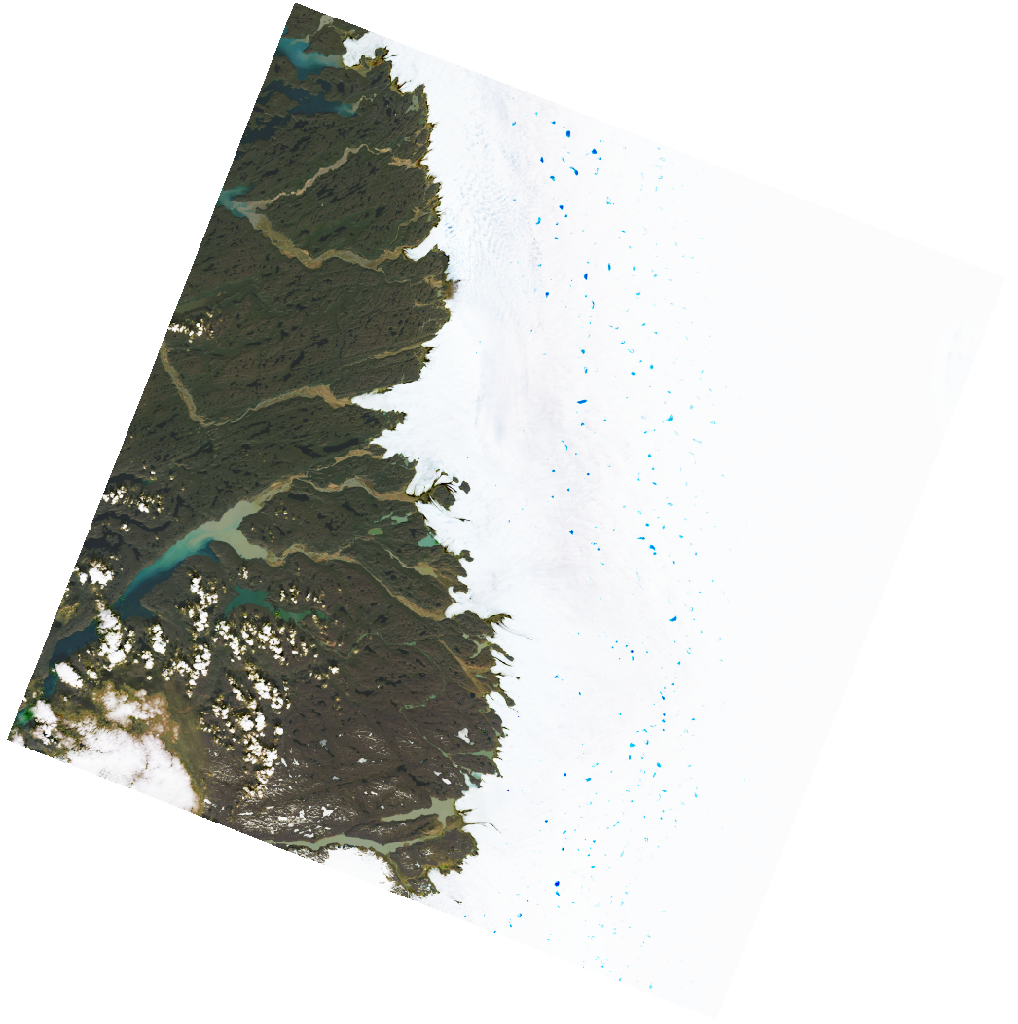
Looks good! We can now get individual bands via the href of their assets, loading with rioxarray. Note that they are not stored in EPSG:4326, they are stored in whatever the appropriate UTM projection is. Therefore, before we clip the data, we must convert our geopandas boundary into the appropriate CRS.
import rioxarray as rxr

# 'Squeeze' is a useful function to remove dimensions of size 1 ('band' in this
# case, as we only have one band, red)
xds = rxr.open_rasterio(item.assets['red'].href).squeeze()

# Note that our data is stored in a UTM projection
print(xds.rio.crs)

# Clip the data, after convertin our geodataframe to the same projection
xds = xds.rio.clip(
    issunguata_gdf_3413.to_crs(xds.rio.crs).geometry.values
)
EPSG:32622
Now, we have got a useful bit of data:
import matplotlib.pyplot as plt

fig, ax = plt.subplots()
xds.plot.imshow(cmap='Greys_r', ax=ax)
issunguata_gdf_3413.to_crs(32622).plot(ax=ax, fc='none', ec='tab:red')
<Axes: title={'center': 'band = 1, spatial_ref = 0'}, xlabel='x coordinate of projection\n[metre]', ylabel='y coordinate of projection\n[metre]'>
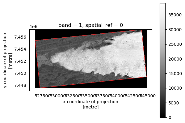
TODO: convert from DN to reflectance. This will also fix the slightly dodgy NDSI values below.
Now, we could go through this charade for every single band we want and stack them together, but there is actually an easier option, using a package called stackstac.
7.3.2. Batch download with stackstac#
stackstac allows us to provide the individual assets we want, a target CRS, target resolution, bounds, and even a method of resampling (which we will do using legacy rasterio function calls). It will provide a single large xarray of all our data, allowing us to pick the dates we want.
issunguata_gdf_3413.to_crs(32622).total_bounds.tolist()
# issunguata_bounds_3413
[526206.6761875935, 7447501.881333968, 544757.4277271645, 7457226.07411013]
import stackstac
from rasterio.enums import Resampling

# Prep our chosen parameters
resampling = Resampling.cubic
assets = ['red', 'green', 'blue', 'swir16']
working_resolution = 30
target_crs = 3413
bounds = issunguata_bounds_3413

# Stack our data
data = stackstac.stack(
    items_aoi_filtered,
    assets=assets,
    resolution=working_resolution,
    epsg=target_crs,
    resampling=resampling,
    bounds=bounds,
    chunksize=512,  # for parallel processing
)

data
<xarray.DataArray 'stackstac-8021831003edc1a707c2bfeb1e58e179' (time: 3,
                                                                band: 4,
                                                                y: 268, x: 601)> Size: 15MB
dask.array<fetch_raster_window, shape=(3, 4, 268, 601), dtype=float64, chunksize=(1, 1, 268, 512), chunktype=numpy.ndarray>
Coordinates: (12/30)
  * time                         (time) datetime64[ns] 24B 2024-05-11T15:00:1...
    id                           (time) <U31 372B 'LC08_L2SP_009012_20240511_...
  * band                         (band) <U6 96B 'red' 'green' 'blue' 'swir16'
  * x                            (x) float64 5kB -2.35e+05 ... -2.17e+05
  * y                            (y) float64 2kB -2.489e+06 ... -2.497e+06
    description                  (band) <U77 1kB 'Collection 2 Level-2 Red Ba...
    ...                           ...
    title                        (band) <U28 448B 'Red Band' ... 'Short-wave ...
    raster:bands                 object 8B {'scale': 2.75e-05, 'nodata': 0, '...
    common_name                  (band) <U6 96B 'red' 'green' 'blue' 'swir16'
    center_wavelength            (band) float64 32B 0.65 0.56 0.48 1.61
    full_width_half_max          (band) float64 32B 0.04 0.06 0.06 0.09
    epsg                         int64 8B 3413
Attributes:
    spec:        RasterSpec(epsg=3413, bounds=(-235020, -2497020, -216990, -2...
    crs:         epsg:3413
    transform:   | 30.00, 0.00,-235020.00|\n| 0.00,-30.00,-2488980.00|\n| 0.0...
resolution: 30Fantastic. You can see our data object is another multidimensional xarray object with four indexes: x, y, band, and time.
It appeared instantly because xarray is still lazily evaluating the data. Let’s get the same dataset again, this time in a slightly different way (why not) by trying to find the specific day from earlier.
scene = data.sel(time="2024-07-16").squeeze()

scene
<xarray.DataArray 'stackstac-8021831003edc1a707c2bfeb1e58e179' (band: 4,
                                                                y: 268, x: 601)> Size: 5MB
dask.array<getitem, shape=(4, 268, 601), dtype=float64, chunksize=(1, 268, 512), chunktype=numpy.ndarray>
Coordinates: (12/30)
    time                         datetime64[ns] 8B 2024-07-16T14:48:33.406055
    id                           <U31 124B 'LC08_L2SP_007013_20240716_02_T1'
  * band                         (band) <U6 96B 'red' 'green' 'blue' 'swir16'
  * x                            (x) float64 5kB -2.35e+05 ... -2.17e+05
  * y                            (y) float64 2kB -2.489e+06 ... -2.497e+06
    description                  (band) <U77 1kB 'Collection 2 Level-2 Red Ba...
    ...                           ...
    title                        (band) <U28 448B 'Red Band' ... 'Short-wave ...
    raster:bands                 object 8B {'scale': 2.75e-05, 'nodata': 0, '...
    common_name                  (band) <U6 96B 'red' 'green' 'blue' 'swir16'
    center_wavelength            (band) float64 32B 0.65 0.56 0.48 1.61
    full_width_half_max          (band) float64 32B 0.04 0.06 0.06 0.09
    epsg                         int64 8B 3413
Attributes:
    spec:        RasterSpec(epsg=3413, bounds=(-235020, -2497020, -216990, -2...
    crs:         epsg:3413
    transform:   | 30.00, 0.00,-235020.00|\n| 0.00,-30.00,-2488980.00|\n| 0.0...
resolution: 30We can now plot the scene - in order to get an RGB plot, we will select only the ['red', 'green', 'blue'] bands in order:
# Force download the scene
scene = scene.compute()

# Get a three-band image
rgb = scene.sel(band=['red', 'green', 'blue'])

# Plot this
fig, ax = plt.subplots()
rgb.plot.imshow(ax=ax)
ax.set_aspect('equal')
Clipping input data to the valid range for imshow with RGB data ([0..1] for floats or [0..255] for integers). Got range [-0.1999725..1.0468775000000001].
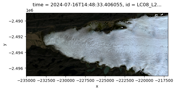
Note that imshow compalined a bit because it expects reflectance values between 0-1 or 8-bit values between 0 and 255. Over ice surfaces with drastic changes in reflectance, you can get values beyond this!
Anyway, let’s do something useful and calculate NDSI! Recall the NDSI equation is
We can work this out as follows:
ndsi = (
    (scene.sel(band='green') - scene.sel(band='swir16'))
    / (scene.sel(band='green') + scene.sel(band='swir16'))
)

fig, ax = plt.subplots()
ndsi.plot.imshow(ax=ax, vmin=-1, vmax=+1, cmap='RdBu')
ax.set_aspect('equal')
plt.show()
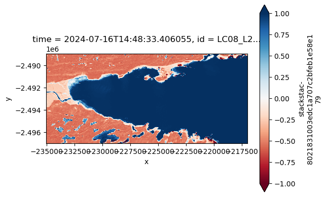
Neat. Remember we can also use other xarray functions to manipulate the data (e.g. getting a long-term average of pixel values).
Most importantly, you might wish to download the data we’ve got in the stack. An example here would look through the stack along the time axis, saving according to the scene ID name. I haven’t set a directory or anything here though.
for i in len(data):

    scene = data.isel(time=i)
    scene_fname = f"{scene.id.item}.tif"
    scene.compute()

    # export cog with zstd compression
    scene.rio.to_raster(scene_fname, driver='COG', compress='zstd')