10. Altimetry Data

(specifically, ICESat-2)

This page is a Jupyter Notebook that can be found and downloaded at the GitHub repository.

Once again, there is no convenient STAC interface for altimetry data. The alternative is nearly as good though - the SlideRule tool has been developed for ICESat-2 (and GEDI) data, which allows you to generate ICESat-2 processed data on the fly.

import pdemtools as pdt 
import geopandas as gpd
import pandas as pd
import matplotlib.pyplot as plt

from sliderule import sliderule, icesat2
from shapely.geometry import box

10.1. SlideRule Example

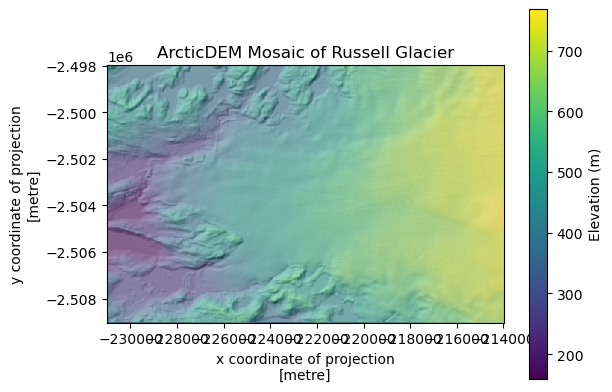
Let’s examine another part of Greenland, and download a bit of the ArcticDEM mosaic for comparison.

russell_bounds = [-231000,-2509000,-214000,-2498000]

russell_gdf_3413 = gpd.GeoDataFrame(geometry=[box(*russell_bounds)], crs=3413)
russell_gdf_4326 = russell_gdf_3413.to_crs(4326)

dem = pdt.load.mosaic('arcticdem', 32, bounds=russell_bounds)
hillshade = dem.pdt.terrain('hillshade')

fig, ax = plt.subplots()

dem.plot.imshow(ax=ax, cbar_kwargs={'label': 'Elevation (m)'})
hillshade.plot.imshow(ax=ax, alpha=0.5, cmap='gray', add_colorbar=False)
ax.set_aspect('equal')
ax.set_title('ArcticDEM Mosaic of Russell Glacier')

Text(0.5, 1.0, 'ArcticDEM Mosaic of Russell Glacier')

Now, let’s show a quick example of how to download ICESat-2 ATL06 data from SlideRule.

# connect to sliderule
icesat2.init("slideruleearth.io")

# Turn the geodataframe into a sliderule-friendly object
sr_region = sliderule.toregion(russell_gdf_4326)

# set search parameters (apart from dates)
params = {
    "poly": sr_region["poly"],
    "t0": "2020-01-01",  # Start date
    "t1": "2020-12-31",  # End date
    "srt": 3,    # Surface. 0-land, 1-ocean, 2-seaice, 3-landice (default), 4-inlandwater
    "cnf": 1,    # Confidence. Default 1 (within 10 m). 2: Low. 3: Medium. 4: High.
    "ats": 20,   # Mininum along track spread. SR Default: 20.
    "cnt": 10,   # Minimum photon count in segment. Default 10.
    "len": 40,   # Extent length. ATL06 default is 40 metres.
    "res": 20,   # Step distance. ATL06 default is 20 metres.
    "track": 0,  # Integer: 0: all tracks, 1: gt1, 2: gt2, 3: gt3. Default 0.
    "sigma_r_max": 5,  # Max robust dispersion [m]. Default 5.
}

is2_gdf = icesat2.atl06p(params).to_crs(3413)

n_points = len(is2_gdf)
print(f"Number of points found: {n_points}")

Warning, this environment is using an outdated client (v4.9.1). The code will run but some functionality supported by the server (v4.19.0) may not be available.

Number of points found: 18537

Now we have our ICESat-2 ATL06 data as a nice geodataframe:

is2_gdf.head()

	h_sigma	rgt	h_mean	w_surface_window_final	y_atc	n_fit_photons	dh_fit_dx	gt	spot	region	rms_misfit	x_atc	pflags	cycle	segment_id	geometry
time
2020-01-10 09:35:06.322201600	0.039076	224	731.273062	3.000000	71.362442	118	0.046058	30	4	5	0.423777	12583511.0	0	6	628250	POINT (-214005.561 -2498259.909)
2020-01-10 09:35:06.325011200	0.057742	224	732.417008	3.881913	71.392601	121	0.055053	30	4	5	0.634964	12583531.0	0	6	628251	POINT (-214009.553 -2498279.699)
2020-01-10 09:35:06.327821824	0.048733	224	732.887001	3.435776	71.412392	131	-0.016056	30	4	5	0.547110	12583551.0	0	6	628252	POINT (-214013.559 -2498299.504)
2020-01-10 09:35:06.330632960	0.025287	224	733.142206	3.000000	71.422310	135	0.048296	30	4	5	0.293369	12583571.0	0	6	628253	POINT (-214017.574 -2498319.306)
2020-01-10 09:35:06.333442816	0.035668	224	733.993594	3.000000	71.423027	105	0.034484	30	4	5	0.363403	12583592.0	0	6	628254	POINT (-214021.598 -2498339.107)

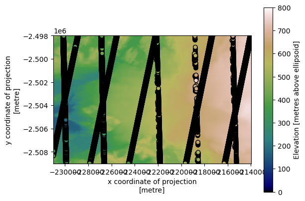
Let’s plot the data to the same colour scale as the ArcticDEM:

fix, ax = plt.subplots()

dem.plot.imshow(ax=ax, cmap='gist_earth', vmin=0, vmax=800, cbar_kwargs={'label': 'Elevation [metres above ellipsoid]'})
is2_gdf.plot(ax=ax, column='h_mean', cmap='gist_earth', vmin=0, vmax=800, ec='k', legend=False)
ax.set_title(None)

plt.show()

Great! Using the geodataframe, you may wish to perform tasks such as filtering to specific dates and crossover points. SlideRule also enables you to download other ICESat-2 derivative data.