Multidimensional Data (xarray)

6.2. Multidimensional Data (`xarray`)#

This page is a Jupyter Notebook that can be found and downloaded at the GitHub repository.

6.2.1. What is multidimensional data?#

Managing more complex data is, of course, slightly more challenging.

You might expect me to jump into 2-D raster data at this point, but we are in fact going to jump into “n-dimensional” climate data (the why will become apparent soon). By n-dimensional, we mean the data can have as many dimensions as we like. Think of a, say, an ERA-5 dataset of atmospheric reanalysis: this gridded dataset will have an x, y, and z dimension, but may also have a time dimension, before we even get to the parameters (pressure, temperature, etc).

If you’ve encountered them before, it’s probably been in a format such as netCDF (.nc) or HDF (.hdf, .h5, etc).

n-dimensional dataset, from https://tutorial.xarray.dev/overview/xarray-in-45-min.html

The community-standard package we use to manage these datasets is called xarray (quickstart tutorial here).

6.2.3. Indexing Datasets#

We can still visualise this, but it’s slightly more complicated. Note that we have our coordinates indices: lat, lon, and time. We also have our air variable, which has data along all three coordinates. (Individual variables don’t need to use every coordinate - imagine there was also an elevation variable, which just used lat and lon but not time).

We can’t plot all of this at once, but we can take slices of the dataset to get an idea of what’s happening. For instance, we could pick a single instance in time:

# Take the 0th index along the time axis, and plot the `air` variable using
# matplotlibs `imshow` in the backend:
xds.isel(time=0).air.plot.imshow()
plt.show()

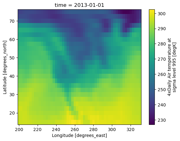
../_images/bd06653e779df297f5a757d7b0213868987603ebdaeaddfb8eebfd8d1f86f909.png

OK, it’s clearer now: this is a temperature record of North America.

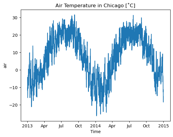
We could, however, try and view this along the time axis. We could choose random indices using isel again, or do something a bit more complex by selecting the pixel closest to a given geographic location:

chicago_lat = 41.8781
chicago_lon = -87.6298 + 360 # data is in positive degrees east, so add 360

# Select nearest grid cell to Chicago
ts_chicago = xds['air'].sel(lat=chicago_lat, lon=chicago_lon, method="nearest")

# ts_chicago is now a DataArray indexed by time, but we could also get a
# pandas dataframe if we wanted using `to_pandas()`

# Air temperature is in Kelvin, so let's convert to Celsius
ts_chicago = ts_chicago - 273.15

# Now let's plot it!

fig, ax = plt.subplots()
ts_chicago.plot(ax=ax)
ax.set_title('Air Temperature in Chicago [˚C]')
plt.show()

../_images/54c342f5258f684d598b0166fcca8b7823860d130279cb969ad7a406f57d1bdd.png

6.2.4. Manipulating Data#

We can go further - what if we wanted the mean July air temperature for the whole of the dataset?

# Get mean July temperature for xds
mean_july = xds['air'].sel(time=xds['time'].dt.month == 7).mean(dim='time')

# Convert to Celsius
mean_july = mean_july - 273.15

# Plot
fig, ax = plt.subplots()
mean_july.plot.imshow(ax=ax)
ax.set_title('Mean July Temperature (2014-2015) [˚C]')
plt.show()

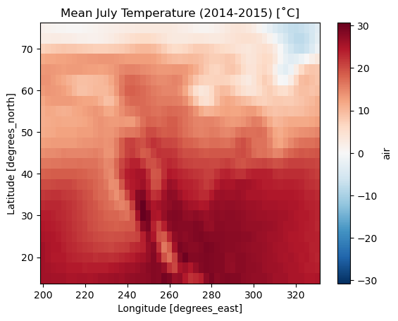
../_images/d6489b2b30e5d2af3107de753ea57587e5ac9982e05cfb5363ffd3325847b123.png

Hopefully this begins to show the strength of how we can use xarray to assess n-dimensional climate datasets.

Multidimensional Data (xarray)

Contents

6.2. Multidimensional Data (`xarray`)#

6.2.1. What is multidimensional data?#

6.2.2. `xarray` Datasets#

6.2.3. Indexing Datasets#

6.2.4. Manipulating Data#

Multidimensional Data (xarray)

Contents

6.2. Multidimensional Data (xarray)#

6.2.1. What is multidimensional data?#

6.2.2. xarray Datasets#

6.2.3. Indexing Datasets#

6.2.4. Manipulating Data#

6.2. Multidimensional Data (`xarray`)#

6.2.2. `xarray` Datasets#