8. Ice Velocity Data#
This page is a Jupyter Notebook that can be found and downloaded at the GitHub repository.
import requests, json

import rioxarray as rxr
import xarray as xr
import geopandas as gpd
import matplotlib.pyplot as plt

from shapely.geometry import box
from typing import Literal, Optional, Union
8.1. Downloading ITS_LIVE mosaic datasets#
The ITS_LIVE mosaic data is hosted on AWS as a series of cloud-optimised GeoTIFFs. Simply find the link to the .tif file you want using the ITS_LIVE GUI and you feed it straight into rioxarray! These are large files so I would recommend applying an AOI - that’s what cloud-optimised data are good for.
Here is a litte function that constructs the file you want for V2 data:
def get_itslive_fpath(
    composite: Optional[bool] = False,
    year: Optional[Union[str, int]] = None,
    variable: Optional[Literal["v", "vx", "vy", "v_error", "vx_error", "vy_error", "count"]] = "v",
    ) -> str:
    """
    Get a filepath to a V2 ITS_LIVE mosaic dataset. Must have either composite
    set to True for the full mosaic, or provide a year.
    """

    if composite == False and year is None:
        raise ValueError("You must set either composite to True or provide a year.")

    if variable not in ["v", "vx", "vy", "v_error", "vx_error", "vy_error", "count"]:
        raise ValueError("variable must be one of 'v', 'vx', 'vy', 'v_error', 'vx_error', 'vy_error', 'count'")

    if composite == True:
        return f"https://its-live-data.s3.amazonaws.com/velocity_mosaic/v2/static/cog/ITS_LIVE_velocity_120m_RGI05A_0000_v02_{variable}.tif"

    else:
        return f"https://its-live-data.s3.amazonaws.com/velocity_mosaic/v2/annual/cog/ITS_LIVE_velocity_120m_RGI05A_{year}_v02_{variable}.tif"
Now we can load some data and display it. I’m going to download both the magnitude data v and the vector vx and vy data so I can show an example of making a simple flow diagram.
The data is in polar stereographic, so I will provide a bounding box accordingly.
vv_fpath = get_itslive_fpath(composite=True, variable="v")
vx_fpath = get_itslive_fpath(composite=True, variable="vx")
vy_fpath = get_itslive_fpath(composite=True, variable="vy")

kangerlussuaq_bounds = 465000, -2300000, 496000, -2258000

vv = rxr.open_rasterio(vv_fpath).rio.clip_box(*kangerlussuaq_bounds).squeeze().compute()
vx = rxr.open_rasterio(vx_fpath).rio.clip_box(*kangerlussuaq_bounds).squeeze().compute()
vy = rxr.open_rasterio(vy_fpath).rio.clip_box(*kangerlussuaq_bounds).squeeze().compute()
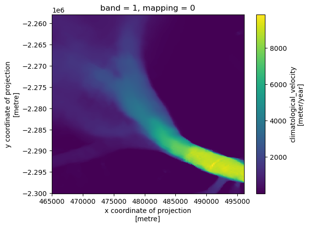
We can easily visualise the velocity field. The composite feild extends into the fjord because of mélange coherence.
vv.plot.imshow()
<matplotlib.image.AxesImage at 0x16b005640>
Let’s make a nice figure:
fig, ax = plt.subplots()

vv.plot.imshow(ax=ax)


show_every = 15  # Show flow direction every n pixels
skip = slice(None, None, show_every)

ax.quiver(
    vv.x.values[skip],
    vv.y.values[skip],
    vx.values[skip, skip],
    vy.values[skip, skip],
    color='white',
    pivot='mid'
)


plt.show()
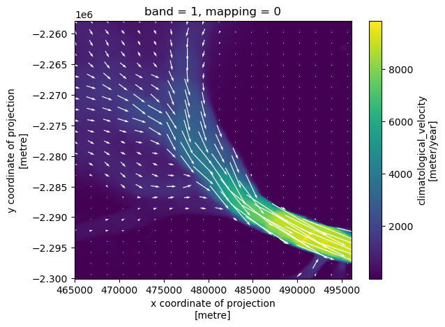
Cool!
8.2. Download Batch Data (the ITS_LIVE zarr file)#
ITS_LIVE also make individual scene-pairs available through cloud datasets. Unfortunately, it isn’t quite as neat as the STAC system, but I’ve put together a relatively hacky way of doing things.
The ITS_LIVE data is split into a series of square ROIs (datacubes) across Greenland. First, we must establish which datacube we need. ITS_LIVE hosts a json catalog of all possible cubes, which can be loaded using geopandas and clipped to your ROI with geopandas.
# generate AOI geodataframe
kangerlussuaq_bounds = 465000, -2300000, 496000, -2258000
aoi_gdf = gpd.GeoDataFrame(
    geometry=[box(*kangerlussuaq_bounds)], crs=3413
)

# load its_live dataset
itslive_url = (
    "https://its-live-data.s3-us-west-2.amazonaws.com/datacubes/catalog_v02.json"
)

with requests.get(itslive_url, stream=True) as response:

    # Check if the request was successful
    if response.status_code == 200:

        json_data = response.text  # Read the JSON data from the response
        data = json.loads(json_data)  # Parse the JSON data into a Python dictionary
        # print(data.keys())

        # Create GeoDataFrame from features
        if data["type"] == "FeatureCollection":
            catalog_gdf = gpd.GeoDataFrame.from_features(data["features"], crs=4326)
        else:
            print("Error: Not a GeoJSON FeatureCollection")

    else:
        print(
            f"Error: Could not retrieve data from URL. Status code: {response.status_code}"
        )

catalog_gdf = catalog_gdf.to_crs(3413)

# clip catalog to AOI
catalog_gdf = catalog_gdf.clip(aoi_gdf)

catalog_gdf
| geometry | fill-opacity | fill | roi_percent_coverage | geometry_epsg | datacube_exist | zarr_url | epsg | granule_count | |
|---|---|---|---|---|---|---|---|---|---|
| 1422 | POLYGON ((465000 -2300000, 465000 -2258000, 49... | 0.0 | red | 100.0 | {'type': 'Polygon', 'coordinates': [[[400000, ... | 1 | http://its-live-data.s3.amazonaws.com/datacube... | 3413 | 77932 |
This is good news! There is only one intersecting zarr file. There is a chance your data could be split across datacubes - this becomes a bit of a pain, and one of the easiest solutions I’ve found it, sadly, to download them both in parallel and stitch two seperate files together when needed. Anyway, now we can simply open the zarr file as an xarray.
zarr_url = catalog_gdf.zarr_url.values[0]
datacube = xr.open_dataset(zarr_url, chunks='auto')
/var/folders/h7/6y8bw0210l5fp4pyvbtkx54r0000gn/T/ipykernel_54245/1836833705.py:2: FutureWarning: In a future version of xarray decode_timedelta will default to False rather than None. To silence this warning, set decode_timedelta to True, False, or a 'CFTimedeltaCoder' instance.
  datacube = xr.open_dataset(zarr_url, chunks='auto')
datacube
<xarray.Dataset> Size: 2TB
Dimensions:                     (mid_date: 80832, y: 833, x: 833)
Coordinates:
  * mid_date                    (mid_date) datetime64[ns] 647kB 2022-01-11T02...
  * x                           (x) float64 7kB 4.001e+05 4.003e+05 ... 5e+05
  * y                           (y) float64 7kB -2.2e+06 -2.2e+06 ... -2.3e+06
Data variables: (12/60)
    M11                         (mid_date, y, x) float32 224GB dask.array<chunksize=(40000, 20, 20), meta=np.ndarray>
    M11_dr_to_vr_factor         (mid_date) float32 323kB dask.array<chunksize=(80832,), meta=np.ndarray>
    M12                         (mid_date, y, x) float32 224GB dask.array<chunksize=(40000, 20, 20), meta=np.ndarray>
    M12_dr_to_vr_factor         (mid_date) float32 323kB dask.array<chunksize=(80832,), meta=np.ndarray>
    acquisition_date_img1       (mid_date) datetime64[ns] 647kB dask.array<chunksize=(80832,), meta=np.ndarray>
    acquisition_date_img2       (mid_date) datetime64[ns] 647kB dask.array<chunksize=(80832,), meta=np.ndarray>
    ...                          ...
    vy_error_modeled            (mid_date) float32 323kB dask.array<chunksize=(80832,), meta=np.ndarray>
    vy_error_slow               (mid_date) float32 323kB dask.array<chunksize=(80832,), meta=np.ndarray>
    vy_error_stationary         (mid_date) float32 323kB dask.array<chunksize=(80832,), meta=np.ndarray>
    vy_stable_shift             (mid_date) float32 323kB dask.array<chunksize=(80832,), meta=np.ndarray>
    vy_stable_shift_slow        (mid_date) float32 323kB dask.array<chunksize=(80832,), meta=np.ndarray>
    vy_stable_shift_stationary  (mid_date) float32 323kB dask.array<chunksize=(80832,), meta=np.ndarray>
Attributes: (12/19)
    Conventions:                CF-1.8
    GDAL_AREA_OR_POINT:         Area
    author:                     ITS_LIVE, a NASA MEaSUREs project (its-live.j...
    autoRIFT_parameter_file:    http://its-live-data.s3.amazonaws.com/autorif...
    datacube_software_version:  1.0
    date_created:               03-Oct-2023 04:39:28
    ...                         ...
    s3:                         s3://its-live-data/datacubes/v2-updated-octob...
    skipped_granules:           s3://its-live-data/datacubes/v2-updated-octob...
    time_standard_img1:         UTC
    time_standard_img2:         UTC
    title:                      ITS_LIVE datacube of image pair velocities
url: https://its-live-data.s3.amazonaws.com/datacu...- mid_date: 80832
- y: 833
- x: 833
- mid_date(mid_date)datetime64[ns]2022-01-11T02:19:00.211010048 .....
- description :
- midpoint of image 1 and image 2 acquisition date and time with granule's centroid longitude and latitude as microseconds
- standard_name :
- image_pair_center_date_with_time_separation
array(['2022-01-11T02:19:00.211010048', '2001-07-18T13:41:52.099001984', '2011-07-30T13:46:04.179220992', ..., '2024-10-26T13:45:57.576919296', '2024-12-24T23:10:23.913507072', '2024-11-27T13:46:28.448804096'], shape=(80832,), dtype='datetime64[ns]') - x(x)float644.001e+05 4.003e+05 ... 5e+05
- description :
- x coordinate of projection
- standard_name :
- projection_x_coordinate
array([400132.5, 400252.5, 400372.5, ..., 499732.5, 499852.5, 499972.5], shape=(833,)) - y(y)float64-2.2e+06 -2.2e+06 ... -2.3e+06
- description :
- y coordinate of projection
- standard_name :
- projection_y_coordinate
array([-2200132.5, -2200252.5, -2200372.5, ..., -2299732.5, -2299852.5,
       -2299972.5], shape=(833,))
- M11(mid_date, y, x)float32dask.array<chunksize=(40000, 20, 20), meta=np.ndarray>
- description :
- conversion matrix element (1st row, 1st column) that can be multiplied with vx to give range pixel displacement dr (see Eq. A18 in https://www.mdpi.com/2072-4292/13/4/749)
- grid_mapping :
- mapping
- standard_name :
- conversion_matrix_element_11
- units :
- pixel/(meter/year)
Array Chunk Bytes 208.95 GiB 62.30 MiB Shape (80832, 833, 833) (40832, 20, 20) Dask graph 3528 chunks in 2 graph layers Data type float32 numpy.ndarray - M11_dr_to_vr_factor(mid_date)float32dask.array<chunksize=(80832,), meta=np.ndarray>
- description :
- multiplicative factor that converts slant range pixel displacement dr to slant range velocity vr
- standard_name :
- M11_dr_to_vr_factor
- units :
- meter/(year*pixel)
Array Chunk Bytes 315.75 kiB 315.75 kiB Shape (80832,) (80832,) Dask graph 1 chunks in 2 graph layers Data type float32 numpy.ndarray - M12(mid_date, y, x)float32dask.array<chunksize=(40000, 20, 20), meta=np.ndarray>
- description :
- conversion matrix element (1st row, 2nd column) that can be multiplied with vy to give range pixel displacement dr (see Eq. A18 in https://www.mdpi.com/2072-4292/13/4/749)
- grid_mapping :
- mapping
- standard_name :
- conversion_matrix_element_12
- units :
- pixel/(meter/year)
Array Chunk Bytes 208.95 GiB 62.30 MiB Shape (80832, 833, 833) (40832, 20, 20) Dask graph 3528 chunks in 2 graph layers Data type float32 numpy.ndarray - M12_dr_to_vr_factor(mid_date)float32dask.array<chunksize=(80832,), meta=np.ndarray>
- description :
- multiplicative factor that converts slant range pixel displacement dr to slant range velocity vr
- standard_name :
- M12_dr_to_vr_factor
- units :
- meter/(year*pixel)
Array Chunk Bytes 315.75 kiB 315.75 kiB Shape (80832,) (80832,) Dask graph 1 chunks in 2 graph layers Data type float32 numpy.ndarray - acquisition_date_img1(mid_date)datetime64[ns]dask.array<chunksize=(80832,), meta=np.ndarray>
- description :
- acquisition date and time of image 1
- standard_name :
- image1_acquition_date
Array Chunk Bytes 631.50 kiB 631.50 kiB Shape (80832,) (80832,) Dask graph 1 chunks in 2 graph layers Data type datetime64[ns] numpy.ndarray - acquisition_date_img2(mid_date)datetime64[ns]dask.array<chunksize=(80832,), meta=np.ndarray>
- description :
- acquisition date and time of image 2
- standard_name :
- image2_acquition_date
Array Chunk Bytes 631.50 kiB 631.50 kiB Shape (80832,) (80832,) Dask graph 1 chunks in 2 graph layers Data type datetime64[ns] numpy.ndarray - autoRIFT_software_version(mid_date)<U5dask.array<chunksize=(80832,), meta=np.ndarray>
- description :
- version of autoRIFT software
- standard_name :
- autoRIFT_software_version
Array Chunk Bytes 1.54 MiB 1.54 MiB Shape (80832,) (80832,) Dask graph 1 chunks in 2 graph layers Data type - chip_size_height(mid_date, y, x)float32dask.array<chunksize=(40000, 20, 20), meta=np.ndarray>
- chip_size_coordinates :
- Optical data: chip_size_coordinates = 'image projection geometry: width = x, height = y'. Radar data: chip_size_coordinates = 'radar geometry: width = range, height = azimuth'
- description :
- height of search template (chip)
- grid_mapping :
- mapping
- standard_name :
- chip_size_height
- units :
- m
- y_pixel_size :
- 10.0
Array Chunk Bytes 208.95 GiB 62.30 MiB Shape (80832, 833, 833) (40832, 20, 20) Dask graph 3528 chunks in 2 graph layers Data type float32 numpy.ndarray - chip_size_width(mid_date, y, x)float32dask.array<chunksize=(40000, 20, 20), meta=np.ndarray>
- chip_size_coordinates :
- Optical data: chip_size_coordinates = 'image projection geometry: width = x, height = y'. Radar data: chip_size_coordinates = 'radar geometry: width = range, height = azimuth'
- description :
- width of search template (chip)
- grid_mapping :
- mapping
- standard_name :
- chip_size_width
- units :
- m
- x_pixel_size :
- 10.0
Array Chunk Bytes 208.95 GiB 62.30 MiB Shape (80832, 833, 833) (40832, 20, 20) Dask graph 3528 chunks in 2 graph layers Data type float32 numpy.ndarray - date_center(mid_date)datetime64[ns]dask.array<chunksize=(80832,), meta=np.ndarray>
- description :
- midpoint of image 1 and image 2 acquisition date
- standard_name :
- image_pair_center_date
Array Chunk Bytes 631.50 kiB 631.50 kiB Shape (80832,) (80832,) Dask graph 1 chunks in 2 graph layers Data type datetime64[ns] numpy.ndarray - date_dt(mid_date)timedelta64[ns]dask.array<chunksize=(80832,), meta=np.ndarray>
- description :
- time separation between acquisition of image 1 and image 2
- standard_name :
- image_pair_time_separation
Array Chunk Bytes 631.50 kiB 631.50 kiB Shape (80832,) (80832,) Dask graph 1 chunks in 2 graph layers Data type timedelta64[ns] numpy.ndarray - floatingice(y, x)float32dask.array<chunksize=(833, 833), meta=np.ndarray>
- description :
- floating ice mask, 0 = non-floating-ice, 1 = floating-ice
- flag_meanings :
- non-ice ice
- flag_values :
- [0, 1]
- grid_mapping :
- mapping
- standard_name :
- floating ice mask
- url :
- https://its-live-data.s3.amazonaws.com/autorift_parameters/v001/NPS_0120m_floatingice.tif
Array Chunk Bytes 2.65 MiB 2.65 MiB Shape (833, 833) (833, 833) Dask graph 1 chunks in 2 graph layers Data type float32 numpy.ndarray - granule_url(mid_date)<U1024dask.array<chunksize=(32732,), meta=np.ndarray>
- description :
- original granule URL
- standard_name :
- granule_url
Array Chunk Bytes 315.75 MiB 127.86 MiB Shape (80832,) (32732,) Dask graph 3 chunks in 2 graph layers Data type - interp_mask(mid_date, y, x)float32dask.array<chunksize=(40000, 20, 20), meta=np.ndarray>
- description :
- light interpolation mask
- flag_meanings :
- measured interpolated
- flag_values :
- [0, 1]
- grid_mapping :
- mapping
- standard_name :
- interpolated_value_mask
Array Chunk Bytes 208.95 GiB 62.30 MiB Shape (80832, 833, 833) (40832, 20, 20) Dask graph 3528 chunks in 2 graph layers Data type float32 numpy.ndarray - landice(y, x)float32dask.array<chunksize=(833, 833), meta=np.ndarray>
- description :
- land ice mask, 0 = non-land-ice, 1 = land-ice
- flag_meanings :
- non-ice ice
- flag_values :
- [0, 1]
- grid_mapping :
- mapping
- standard_name :
- land ice mask
- url :
- https://its-live-data.s3.amazonaws.com/autorift_parameters/v001/NPS_0120m_landice.tif
Array Chunk Bytes 2.65 MiB 2.65 MiB Shape (833, 833) (833, 833) Dask graph 1 chunks in 2 graph layers Data type float32 numpy.ndarray - mapping()<U1...
- GeoTransform :
- 400072.5 120.0 0 -2200072.5 0 -120.0
- crs_wkt :
- PROJCS["WGS 84 / NSIDC Sea Ice Polar Stereographic North",GEOGCS["WGS 84",DATUM["WGS_1984",SPHEROID["WGS 84",6378137,298.257223563,AUTHORITY["EPSG","7030"]],AUTHORITY["EPSG","6326"]],PRIMEM["Greenwich",0,AUTHORITY["EPSG","8901"]],UNIT["degree",0.0174532925199433,AUTHORITY["EPSG","9122"]],AUTHORITY["EPSG","4326"]],PROJECTION["Polar_Stereographic"],PARAMETER["latitude_of_origin",70],PARAMETER["central_meridian",-45],PARAMETER["false_easting",0],PARAMETER["false_northing",0],UNIT["metre",1,AUTHORITY["EPSG","9001"]],AXIS["Easting",SOUTH],AXIS["Northing",SOUTH],AUTHORITY["EPSG","3413"]]
- false_easting :
- 0.0
- false_northing :
- 0.0
- grid_mapping_name :
- polar_stereographic
- inverse_flattening :
- 298.257223563
- latitude_of_origin :
- 70.0
- latitude_of_projection_origin :
- 90.0
- proj4text :
- +proj=stere +lat_0=90 +lat_ts=70 +lon_0=-45 +x_0=0 +y_0=0 +datum=WGS84 +units=m +no_defs
- scale_factor_at_projection_origin :
- 1
- semi_major_axis :
- 6378137.0
- spatial_epsg :
- 3413
- spatial_ref :
- PROJCS["WGS 84 / NSIDC Sea Ice Polar Stereographic North",GEOGCS["WGS 84",DATUM["WGS_1984",SPHEROID["WGS 84",6378137,298.257223563,AUTHORITY["EPSG","7030"]],AUTHORITY["EPSG","6326"]],PRIMEM["Greenwich",0,AUTHORITY["EPSG","8901"]],UNIT["degree",0.0174532925199433,AUTHORITY["EPSG","9122"]],AUTHORITY["EPSG","4326"]],PROJECTION["Polar_Stereographic"],PARAMETER["latitude_of_origin",70],PARAMETER["central_meridian",-45],PARAMETER["false_easting",0],PARAMETER["false_northing",0],UNIT["metre",1,AUTHORITY["EPSG","9001"]],AXIS["Easting",SOUTH],AXIS["Northing",SOUTH],AUTHORITY["EPSG","3413"]]
- straight_vertical_longitude_from_pole :
- -45.0
[1 values with dtype=<U1]
- mission_img1(mid_date)<U1dask.array<chunksize=(80832,), meta=np.ndarray>
- description :
- id of the mission that acquired image 1
- standard_name :
- image1_mission
Array Chunk Bytes 315.75 kiB 315.75 kiB Shape (80832,) (80832,) Dask graph 1 chunks in 2 graph layers Data type - mission_img2(mid_date)<U1dask.array<chunksize=(80832,), meta=np.ndarray>
- description :
- id of the mission that acquired image 2
- standard_name :
- image2_mission
Array Chunk Bytes 315.75 kiB 315.75 kiB Shape (80832,) (80832,) Dask graph 1 chunks in 2 graph layers Data type - roi_valid_percentage(mid_date)float32dask.array<chunksize=(80832,), meta=np.ndarray>
- description :
- percentage of pixels with a valid velocity estimate determined for the intersection of the full image pair footprint and the region of interest (roi) that defines where autoRIFT tried to estimate a velocity
- standard_name :
- region_of_interest_valid_pixel_percentage
Array Chunk Bytes 315.75 kiB 315.75 kiB Shape (80832,) (80832,) Dask graph 1 chunks in 2 graph layers Data type float32 numpy.ndarray - satellite_img1(mid_date)<U2dask.array<chunksize=(80832,), meta=np.ndarray>
- description :
- id of the satellite that acquired image 1
- standard_name :
- image1_satellite
Array Chunk Bytes 631.50 kiB 631.50 kiB Shape (80832,) (80832,) Dask graph 1 chunks in 2 graph layers Data type - satellite_img2(mid_date)<U2dask.array<chunksize=(80832,), meta=np.ndarray>
- description :
- id of the satellite that acquired image 2
- standard_name :
- image2_satellite
Array Chunk Bytes 631.50 kiB 631.50 kiB Shape (80832,) (80832,) Dask graph 1 chunks in 2 graph layers Data type - sensor_img1(mid_date)<U3dask.array<chunksize=(80832,), meta=np.ndarray>
- description :
- id of the sensor that acquired image 1
- standard_name :
- image1_sensor
Array Chunk Bytes 0.93 MiB 0.93 MiB Shape (80832,) (80832,) Dask graph 1 chunks in 2 graph layers Data type - sensor_img2(mid_date)<U3dask.array<chunksize=(80832,), meta=np.ndarray>
- description :
- id of the sensor that acquired image 2
- standard_name :
- image2_sensor
Array Chunk Bytes 0.93 MiB 0.93 MiB Shape (80832,) (80832,) Dask graph 1 chunks in 2 graph layers Data type - stable_count_slow(mid_date)uint16dask.array<chunksize=(80832,), meta=np.ndarray>
- description :
- number of valid pixels over slowest 25% of ice
- standard_name :
- stable_count_slow
- units :
- count
Array Chunk Bytes 157.88 kiB 157.88 kiB Shape (80832,) (80832,) Dask graph 1 chunks in 2 graph layers Data type uint16 numpy.ndarray - stable_count_stationary(mid_date)uint16dask.array<chunksize=(80832,), meta=np.ndarray>
- description :
- number of valid pixels over stationary or slow-flowing surfaces
- standard_name :
- stable_count_stationary
- units :
- count
Array Chunk Bytes 157.88 kiB 157.88 kiB Shape (80832,) (80832,) Dask graph 1 chunks in 2 graph layers Data type uint16 numpy.ndarray - stable_shift_flag(mid_date)uint8dask.array<chunksize=(80832,), meta=np.ndarray>
- description :
- flag for applying velocity bias correction: 0 = no correction; 1 = correction from overlapping stable surface mask (stationary or slow-flowing surfaces with velocity < 15 m/yr)(top priority); 2 = correction from slowest 25% of overlapping velocities (second priority)
- standard_name :
- stable_shift_flag
Array Chunk Bytes 78.94 kiB 78.94 kiB Shape (80832,) (80832,) Dask graph 1 chunks in 2 graph layers Data type uint8 numpy.ndarray - v(mid_date, y, x)float32dask.array<chunksize=(40000, 20, 20), meta=np.ndarray>
- description :
- velocity magnitude
- grid_mapping :
- mapping
- standard_name :
- land_ice_surface_velocity
- units :
- meter/year
Array Chunk Bytes 208.95 GiB 62.30 MiB Shape (80832, 833, 833) (40832, 20, 20) Dask graph 3528 chunks in 2 graph layers Data type float32 numpy.ndarray - v_error(mid_date, y, x)float32dask.array<chunksize=(40000, 20, 20), meta=np.ndarray>
- description :
- velocity magnitude error
- grid_mapping :
- mapping
- standard_name :
- velocity_error
- units :
- meter/year
Array Chunk Bytes 208.95 GiB 62.30 MiB Shape (80832, 833, 833) (40832, 20, 20) Dask graph 3528 chunks in 2 graph layers Data type float32 numpy.ndarray - va(mid_date, y, x)float32dask.array<chunksize=(40000, 20, 20), meta=np.ndarray>
- description :
- velocity in radar azimuth direction
- grid_mapping :
- mapping
Array Chunk Bytes 208.95 GiB 62.30 MiB Shape (80832, 833, 833) (40832, 20, 20) Dask graph 3528 chunks in 2 graph layers Data type float32 numpy.ndarray - va_error(mid_date)float32dask.array<chunksize=(80832,), meta=np.ndarray>
- description :
- error for velocity in radar azimuth direction
- standard_name :
- va_error
- units :
- meter/year
Array Chunk Bytes 315.75 kiB 315.75 kiB Shape (80832,) (80832,) Dask graph 1 chunks in 2 graph layers Data type float32 numpy.ndarray - va_error_modeled(mid_date)float32dask.array<chunksize=(80832,), meta=np.ndarray>
- description :
- 1-sigma error calculated using a modeled error-dt relationship
- standard_name :
- va_error_modeled
- units :
- meter/year
Array Chunk Bytes 315.75 kiB 315.75 kiB Shape (80832,) (80832,) Dask graph 1 chunks in 2 graph layers Data type float32 numpy.ndarray - va_error_slow(mid_date)float32dask.array<chunksize=(80832,), meta=np.ndarray>
- description :
- RMSE over slowest 25% of retrieved velocities
- standard_name :
- va_error_slow
- units :
- meter/year
Array Chunk Bytes 315.75 kiB 315.75 kiB Shape (80832,) (80832,) Dask graph 1 chunks in 2 graph layers Data type float32 numpy.ndarray - va_error_stationary(mid_date)float32dask.array<chunksize=(80832,), meta=np.ndarray>
- description :
- RMSE over stable surfaces, stationary or slow-flowing surfaces with velocity < 15 m/yr identified from an external mask
- standard_name :
- va_error_stationary
- units :
- meter/year
Array Chunk Bytes 315.75 kiB 315.75 kiB Shape (80832,) (80832,) Dask graph 1 chunks in 2 graph layers Data type float32 numpy.ndarray - va_stable_shift(mid_date)float32dask.array<chunksize=(80832,), meta=np.ndarray>
- description :
- applied va shift calibrated using pixels over stable or slow surfaces
- standard_name :
- va_stable_shift
- units :
- meter/year
Array Chunk Bytes 315.75 kiB 315.75 kiB Shape (80832,) (80832,) Dask graph 1 chunks in 2 graph layers Data type float32 numpy.ndarray - va_stable_shift_slow(mid_date)float32dask.array<chunksize=(80832,), meta=np.ndarray>
- description :
- va shift calibrated using valid pixels over slowest 25% of retrieved velocities
- standard_name :
- va_stable_shift_slow
- units :
- meter/year
Array Chunk Bytes 315.75 kiB 315.75 kiB Shape (80832,) (80832,) Dask graph 1 chunks in 2 graph layers Data type float32 numpy.ndarray - va_stable_shift_stationary(mid_date)float32dask.array<chunksize=(80832,), meta=np.ndarray>
- description :
- va shift calibrated using valid pixels over stable surfaces, stationary or slow-flowing surfaces with velocity < 15 m/yr identified from an external mask
- standard_name :
- va_stable_shift_stationary
- units :
- meter/year
Array Chunk Bytes 315.75 kiB 315.75 kiB Shape (80832,) (80832,) Dask graph 1 chunks in 2 graph layers Data type float32 numpy.ndarray - vr(mid_date, y, x)float32dask.array<chunksize=(40000, 20, 20), meta=np.ndarray>
- description :
- velocity in radar range direction
- grid_mapping :
- mapping
Array Chunk Bytes 208.95 GiB 62.30 MiB Shape (80832, 833, 833) (40832, 20, 20) Dask graph 3528 chunks in 2 graph layers Data type float32 numpy.ndarray - vr_error(mid_date)float32dask.array<chunksize=(80832,), meta=np.ndarray>
- description :
- error for velocity in radar range direction
- standard_name :
- vr_error
- units :
- meter/year
Array Chunk Bytes 315.75 kiB 315.75 kiB Shape (80832,) (80832,) Dask graph 1 chunks in 2 graph layers Data type float32 numpy.ndarray - vr_error_modeled(mid_date)float32dask.array<chunksize=(80832,), meta=np.ndarray>
- description :
- 1-sigma error calculated using a modeled error-dt relationship
- standard_name :
- vr_error_modeled
- units :
- meter/year
Array Chunk Bytes 315.75 kiB 315.75 kiB Shape (80832,) (80832,) Dask graph 1 chunks in 2 graph layers Data type float32 numpy.ndarray - vr_error_slow(mid_date)float32dask.array<chunksize=(80832,), meta=np.ndarray>
- description :
- RMSE over slowest 25% of retrieved velocities
- standard_name :
- vr_error_slow
- units :
- meter/year
Array Chunk Bytes 315.75 kiB 315.75 kiB Shape (80832,) (80832,) Dask graph 1 chunks in 2 graph layers Data type float32 numpy.ndarray - vr_error_stationary(mid_date)float32dask.array<chunksize=(80832,), meta=np.ndarray>
- description :
- RMSE over stable surfaces, stationary or slow-flowing surfaces with velocity < 15 m/yr identified from an external mask
- standard_name :
- vr_error_stationary
- units :
- meter/year
Array Chunk Bytes 315.75 kiB 315.75 kiB Shape (80832,) (80832,) Dask graph 1 chunks in 2 graph layers Data type float32 numpy.ndarray - vr_stable_shift(mid_date)float32dask.array<chunksize=(80832,), meta=np.ndarray>
- description :
- applied vr shift calibrated using pixels over stable or slow surfaces
- standard_name :
- vr_stable_shift
- units :
- meter/year
Array Chunk Bytes 315.75 kiB 315.75 kiB Shape (80832,) (80832,) Dask graph 1 chunks in 2 graph layers Data type float32 numpy.ndarray - vr_stable_shift_slow(mid_date)float32dask.array<chunksize=(80832,), meta=np.ndarray>
- description :
- vr shift calibrated using valid pixels over slowest 25% of retrieved velocities
- standard_name :
- vr_stable_shift_slow
- units :
- meter/year
Array Chunk Bytes 315.75 kiB 315.75 kiB Shape (80832,) (80832,) Dask graph 1 chunks in 2 graph layers Data type float32 numpy.ndarray - vr_stable_shift_stationary(mid_date)float32dask.array<chunksize=(80832,), meta=np.ndarray>
- description :
- vr shift calibrated using valid pixels over stable surfaces, stationary or slow-flowing surfaces with velocity < 15 m/yr identified from an external mask
- standard_name :
- vr_stable_shift_stationary
- units :
- meter/year
Array Chunk Bytes 315.75 kiB 315.75 kiB Shape (80832,) (80832,) Dask graph 1 chunks in 2 graph layers Data type float32 numpy.ndarray - vx(mid_date, y, x)float32dask.array<chunksize=(40000, 20, 20), meta=np.ndarray>
- description :
- velocity component in x direction
- grid_mapping :
- mapping
- standard_name :
- land_ice_surface_x_velocity
- units :
- meter/year
Array Chunk Bytes 208.95 GiB 62.30 MiB Shape (80832, 833, 833) (40832, 20, 20) Dask graph 3528 chunks in 2 graph layers Data type float32 numpy.ndarray - vx_error(mid_date)float32dask.array<chunksize=(80832,), meta=np.ndarray>
- description :
- best estimate of x_velocity error: vx_error is populated according to the approach used for the velocity bias correction as indicated in "stable_shift_flag"
- standard_name :
- vx_error
- units :
- meter/year
Array Chunk Bytes 315.75 kiB 315.75 kiB Shape (80832,) (80832,) Dask graph 1 chunks in 2 graph layers Data type float32 numpy.ndarray - vx_error_modeled(mid_date)float32dask.array<chunksize=(80832,), meta=np.ndarray>
- description :
- 1-sigma error calculated using a modeled error-dt relationship
- standard_name :
- vx_error_modeled
- units :
- meter/year
Array Chunk Bytes 315.75 kiB 315.75 kiB Shape (80832,) (80832,) Dask graph 1 chunks in 2 graph layers Data type float32 numpy.ndarray - vx_error_slow(mid_date)float32dask.array<chunksize=(80832,), meta=np.ndarray>
- description :
- RMSE over slowest 25% of retrieved velocities
- standard_name :
- vx_error_slow
- units :
- meter/year
Array Chunk Bytes 315.75 kiB 315.75 kiB Shape (80832,) (80832,) Dask graph 1 chunks in 2 graph layers Data type float32 numpy.ndarray - vx_error_stationary(mid_date)float32dask.array<chunksize=(80832,), meta=np.ndarray>
- description :
- RMSE over stable surfaces, stationary or slow-flowing surfaces with velocity < 15 meter/year identified from an external mask
- standard_name :
- vx_error_stationary
- units :
- meter/year
Array Chunk Bytes 315.75 kiB 315.75 kiB Shape (80832,) (80832,) Dask graph 1 chunks in 2 graph layers Data type float32 numpy.ndarray - vx_stable_shift(mid_date)float32dask.array<chunksize=(80832,), meta=np.ndarray>
- description :
- applied vx shift calibrated using pixels over stable or slow surfaces
- standard_name :
- vx_stable_shift
- units :
- meter/year
Array Chunk Bytes 315.75 kiB 315.75 kiB Shape (80832,) (80832,) Dask graph 1 chunks in 2 graph layers Data type float32 numpy.ndarray - vx_stable_shift_slow(mid_date)float32dask.array<chunksize=(80832,), meta=np.ndarray>
- description :
- vx shift calibrated using valid pixels over slowest 25% of retrieved velocities
- standard_name :
- vx_stable_shift_slow
- units :
- meter/year
Array Chunk Bytes 315.75 kiB 315.75 kiB Shape (80832,) (80832,) Dask graph 1 chunks in 2 graph layers Data type float32 numpy.ndarray - vx_stable_shift_stationary(mid_date)float32dask.array<chunksize=(80832,), meta=np.ndarray>
- description :
- vx shift calibrated using valid pixels over stable surfaces, stationary or slow-flowing surfaces with velocity < 15 m/yr identified from an external mask
- standard_name :
- vx_stable_shift_stationary
- units :
- meter/year
Array Chunk Bytes 315.75 kiB 315.75 kiB Shape (80832,) (80832,) Dask graph 1 chunks in 2 graph layers Data type float32 numpy.ndarray - vy(mid_date, y, x)float32dask.array<chunksize=(40000, 20, 20), meta=np.ndarray>
- description :
- velocity component in y direction
- grid_mapping :
- mapping
- standard_name :
- land_ice_surface_y_velocity
- units :
- meter/year
Array Chunk Bytes 208.95 GiB 62.30 MiB Shape (80832, 833, 833) (40832, 20, 20) Dask graph 3528 chunks in 2 graph layers Data type float32 numpy.ndarray - vy_error(mid_date)float32dask.array<chunksize=(80832,), meta=np.ndarray>
- description :
- best estimate of y_velocity error: vy_error is populated according to the approach used for the velocity bias correction as indicated in "stable_shift_flag"
- standard_name :
- vy_error
- units :
- meter/year
Array Chunk Bytes 315.75 kiB 315.75 kiB Shape (80832,) (80832,) Dask graph 1 chunks in 2 graph layers Data type float32 numpy.ndarray - vy_error_modeled(mid_date)float32dask.array<chunksize=(80832,), meta=np.ndarray>
- description :
- 1-sigma error calculated using a modeled error-dt relationship
- standard_name :
- vy_error_modeled
- units :
- meter/year
Array Chunk Bytes 315.75 kiB 315.75 kiB Shape (80832,) (80832,) Dask graph 1 chunks in 2 graph layers Data type float32 numpy.ndarray - vy_error_slow(mid_date)float32dask.array<chunksize=(80832,), meta=np.ndarray>
- description :
- RMSE over slowest 25% of retrieved velocities
- standard_name :
- vy_error_slow
- units :
- meter/year
Array Chunk Bytes 315.75 kiB 315.75 kiB Shape (80832,) (80832,) Dask graph 1 chunks in 2 graph layers Data type float32 numpy.ndarray - vy_error_stationary(mid_date)float32dask.array<chunksize=(80832,), meta=np.ndarray>
- description :
- RMSE over stable surfaces, stationary or slow-flowing surfaces with velocity < 15 meter/year identified from an external mask
- standard_name :
- vy_error_stationary
- units :
- meter/year
Array Chunk Bytes 315.75 kiB 315.75 kiB Shape (80832,) (80832,) Dask graph 1 chunks in 2 graph layers Data type float32 numpy.ndarray - vy_stable_shift(mid_date)float32dask.array<chunksize=(80832,), meta=np.ndarray>
- description :
- applied vy shift calibrated using pixels over stable or slow surfaces
- standard_name :
- vy_stable_shift
- units :
- meter/year
Array Chunk Bytes 315.75 kiB 315.75 kiB Shape (80832,) (80832,) Dask graph 1 chunks in 2 graph layers Data type float32 numpy.ndarray - vy_stable_shift_slow(mid_date)float32dask.array<chunksize=(80832,), meta=np.ndarray>
- description :
- vy shift calibrated using valid pixels over slowest 25% of retrieved velocities
- standard_name :
- vy_stable_shift_slow
- units :
- meter/year
Array Chunk Bytes 315.75 kiB 315.75 kiB Shape (80832,) (80832,) Dask graph 1 chunks in 2 graph layers Data type float32 numpy.ndarray - vy_stable_shift_stationary(mid_date)float32dask.array<chunksize=(80832,), meta=np.ndarray>
- description :
- vy shift calibrated using valid pixels over stable surfaces, stationary or slow-flowing surfaces with velocity < 15 m/yr identified from an external mask
- standard_name :
- vy_stable_shift_stationary
- units :
- meter/year
Array Chunk Bytes 315.75 kiB 315.75 kiB Shape (80832,) (80832,) Dask graph 1 chunks in 2 graph layers Data type float32 numpy.ndarray
- mid_datePandasIndex
PandasIndex(DatetimeIndex(['2022-01-11 02:19:00.211010048', '2001-07-18 13:41:52.099001984', '2011-07-30 13:46:04.179220992', '2022-04-28 02:09:20.220224', '2021-09-20 14:18:24.210909952', '2010-06-01 13:45:09.167776', '2022-07-07 02:09:10.220505088', '1999-12-13 13:39:27.427602048', '2019-12-30 14:17:44.190622976', '1987-02-20 13:04:48.218380992', ... '2024-11-25 13:58:17.807232', '2024-02-29 13:46:37.747235072', '2024-04-17 13:46:28.253056', '2025-01-03 13:40:21.822998016', '2024-09-12 13:46:32.125246976', '2024-11-30 13:52:52.726549760', '2024-12-04 13:52:41.272830976', '2024-10-26 13:45:57.576919296', '2024-12-24 23:10:23.913507072', '2024-11-27 13:46:28.448804096'], dtype='datetime64[ns]', name='mid_date', length=80832, freq=None)) - xPandasIndex
PandasIndex(Index([400132.5, 400252.5, 400372.5, 400492.5, 400612.5, 400732.5, 400852.5, 400972.5, 401092.5, 401212.5, ... 498892.5, 499012.5, 499132.5, 499252.5, 499372.5, 499492.5, 499612.5, 499732.5, 499852.5, 499972.5], dtype='float64', name='x', length=833)) - yPandasIndex
PandasIndex(Index([-2200132.5, -2200252.5, -2200372.5, -2200492.5, -2200612.5, -2200732.5,
       -2200852.5, -2200972.5, -2201092.5, -2201212.5,
       ...
       -2298892.5, -2299012.5, -2299132.5, -2299252.5, -2299372.5, -2299492.5,
       -2299612.5, -2299732.5, -2299852.5, -2299972.5],
      dtype='float64', name='y', length=833))
- Conventions :
- CF-1.8
- GDAL_AREA_OR_POINT :
- Area
- author :
- ITS_LIVE, a NASA MEaSUREs project (its-live.jpl.nasa.gov)
- autoRIFT_parameter_file :
- http://its-live-data.s3.amazonaws.com/autorift_parameters/v001/autorift_landice_0120m.shp
- datacube_software_version :
- 1.0
- date_created :
- 03-Oct-2023 04:39:28
- date_updated :
- 20-Jun-2025 00:14:51
- geo_polygon :
- [[-35.13419305691563, 68.68857743650318], [-34.530825742288584, 68.6491799734919], [-33.92979742206064, 68.6074812111573], [-33.33122599963105, 68.56349583427193], [-32.7352262721076, 68.5172392115442], [-32.604593166241536, 68.73524065751918], [-32.47119229084849, 68.95328163759716], [-32.33493623495764, 69.17135699618164], [-32.195733934713246, 69.38946141496614], [-32.816343414012614, 69.43785576586481], [-33.43986920578223, 69.48388272309275], [-34.06618321424421, 69.52752492224161], [-34.69515353123396, 69.56876575655875], [-34.80849814997231, 69.34860834881333], [-34.91940201245768, 69.12852181021536], [-35.02794231266891, 68.9085101930343], [-35.13419305691563, 68.68857743650318]]
- institution :
- NASA Jet Propulsion Laboratory (JPL), California Institute of Technology
- latitude :
- 69.05
- longitude :
- -33.69
- proj_polygon :
- [[400000, -2300000], [425000.0, -2300000.0], [450000.0, -2300000.0], [475000.0, -2300000.0], [500000, -2300000], [500000.0, -2275000.0], [500000.0, -2250000.0], [500000.0, -2225000.0], [500000, -2200000], [475000.0, -2200000.0], [450000.0, -2200000.0], [425000.0, -2200000.0], [400000, -2200000], [400000.0, -2225000.0], [400000.0, -2250000.0], [400000.0, -2275000.0], [400000, -2300000]]
- projection :
- 3413
- s3 :
- s3://its-live-data/datacubes/v2-updated-october2024/N60W030/ITS_LIVE_vel_EPSG3413_G0120_X450000_Y-2250000.zarr
- skipped_granules :
- s3://its-live-data/datacubes/v2-updated-october2024/N60W030/ITS_LIVE_vel_EPSG3413_G0120_X450000_Y-2250000.json
- time_standard_img1 :
- UTC
- time_standard_img2 :
- UTC
- title :
- ITS_LIVE datacube of image pair velocities
- url :
- https://its-live-data.s3.amazonaws.com/datacubes/v2-updated-october2024/N60W030/ITS_LIVE_vel_EPSG3413_G0120_X450000_Y-2250000.zarr
As you can see, we now have an xarray dataset with dimensions x, y, and mid_date. There’s a huge amount of data variables and it’s worth stripping this down before downloading anything - explicitly select only variables you understand and want. You might wish to filter by mid_date, date_dt, etc. etc.
8.3. Calculate Derivative Strain Rates#
I have a further Python package strain_tools (NB: this may not be public yet) which enables you to conveniently calculate strain rates from vx and vy data. Documentation is available at the repo.