11. Discharge Data#
import requests

import pandas as pd
import matplotlib.pyplot as plt

from bs4 import BeautifulSoup
Greenland discharge data is readily available to download from the cloud from Ken Mankoff’s Greenland Ice Sheet solid ice discharge from 1986 through last month dataset.
The most recent paper citation is:
Mankoff, K. D., Solgaard, A., Colgan, W., Ahlstrøm, A. P., Khan, S. A., & Fausto, R. S. (2020). Greenland Ice Sheet solid ice discharge from 1986 through March 2020. Earth System Science Data, 12(2), 1367-1383. https://doi.org/10.5194/essd-12-1367-2020
And the dataset can be found at:
Mankoff, K. D., Solgaard, A., & Larsen, S. (2020). Greenland Ice Sheet solid ice discharge from 1986 through last month: Discharge, GEUS Dataverse https://doi.org/10.22008/promice/data/ice_discharge/d/v02
The dataset updates monthly with new discharge data and a new version. As well as the GEUS dataverse page, there is a specific page that always links to the most recent versions of the dataset, located at https://dataverse.geus.dk/api/datasets/:persistentId/dirindex?persistentId=doi:10.22008/promice/data/ice_discharge/d/v02.
12. Downloading Data#
We can use this page to write a simple function that will get direct links to the most recent CSVs. This uses the standard library requests package, as well as “Beautiful Soup”, a popular library for parsing HTML (i.e. web markup language).
def get_discharge_links():
    url = 'https://dataverse.geus.dk/api/datasets/:persistentId/dirindex?persistentId=doi:10.22008/promice/data/ice_discharge/d/v02'
    html = requests.get(url).text
    soup = BeautifulSoup(html, 'html.parser')
    return {a.text.strip(): "https://dataverse.geus.dk" + a["href"] for a in soup.find_all("a")}

links = get_discharge_links()
We now have a complete dictionary of the links, which I print out below.
links
{'gate.nc': 'https://dataverse.geus.dk/api/access/datafile/93550',
 'gate_coverage.csv': 'https://dataverse.geus.dk/api/access/datafile/93547',
 'gate_D.csv': 'https://dataverse.geus.dk/api/access/datafile/93548',
 'gate_err.csv': 'https://dataverse.geus.dk/api/access/datafile/93549',
 'gate_meta.csv': 'https://dataverse.geus.dk/api/access/datafile/78366',
 'GIS.nc': 'https://dataverse.geus.dk/api/access/datafile/93554',
 'GIS_coverage.csv': 'https://dataverse.geus.dk/api/access/datafile/93551',
 'GIS_D.csv': 'https://dataverse.geus.dk/api/access/datafile/93552',
 'GIS_err.csv': 'https://dataverse.geus.dk/api/access/datafile/93553',
 'README.txt': 'https://dataverse.geus.dk/api/access/datafile/93146',
 'region.nc': 'https://dataverse.geus.dk/api/access/datafile/93558',
 'region_coverage.csv': 'https://dataverse.geus.dk/api/access/datafile/93555',
 'region_D.csv': 'https://dataverse.geus.dk/api/access/datafile/93556',
 'region_err.csv': 'https://dataverse.geus.dk/api/access/datafile/93557',
 'sector.nc': 'https://dataverse.geus.dk/api/access/datafile/93562',
 'sector_coverage.csv': 'https://dataverse.geus.dk/api/access/datafile/93559',
 'sector_D.csv': 'https://dataverse.geus.dk/api/access/datafile/93560',
 'sector_err.csv': 'https://dataverse.geus.dk/api/access/datafile/93561'}
The README.txt outlines what each of the files are:
Filename |
Description |
|---|---|
|
Greenland Ice Sheet cumulative discharge by timestamp |
|
Errors for GIS_D.csv |
|
Coverage for GIS_D.csv |
|
Discharge, errors, and coverage for GIS |
|
Regional discharge |
|
Errors for region_D.csv |
|
Coverage for region_D.csv |
|
Discharge, errors, and coverage for GIS regions |
|
Sector discharge |
|
Errors for sector_D.csv |
|
Coverage for sector_D.csv |
|
Discharge, errors, and coverage for GIS sectors |
|
Gate discharge |
|
Errors for gate_D.csv |
|
Coverage for gate_D.csv |
|
Discharge, errors, and coverage for GIS gates - including gate metadata |
|
Metadata for each gate |
We can load the .csv files directly using Pandas, and begin to play.
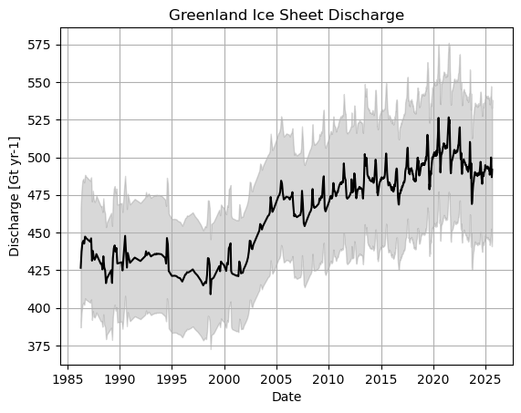
12.1. Greenland-wide Discharge#
gis_d_df = pd.read_csv(links['GIS_D.csv'], parse_dates=['Date'])
gis_err_df = pd.read_csv(links['GIS_err.csv'], parse_dates=['Date'])
gis_df = pd.merge(gis_d_df, gis_err_df, on='Date', how='inner')

gis_df
| Date | Discharge [Gt yr-1] | Discharge Error [Gt yr-1] | |
|---|---|---|---|
| 0 | 1986-04-15 | 426.529 | 39.572 |
| 1 | 1986-05-15 | 437.313 | 40.547 |
| 2 | 1986-06-15 | 443.186 | 41.209 |
| 3 | 1986-07-15 | 444.473 | 41.196 |
| 4 | 1986-08-15 | 442.602 | 40.659 |
| ... | ... | ... | ... |
| 2920 | 2025-07-03 | 494.212 | 46.926 |
| 2921 | 2025-07-15 | 499.877 | 47.389 |
| 2922 | 2025-07-27 | 491.225 | 46.367 |
| 2923 | 2025-08-08 | 486.759 | 45.928 |
| 2924 | 2025-08-20 | 491.769 | 46.459 |
2925 rows × 3 columns
fig, ax = plt.subplots()

# ax.errorbar(gis_df['Date'], gis_df['Discharge [Gt yr-1]'], yerr=gis_df['Discharge Error [Gt yr-1]'], capsize=5)

ax.plot(gis_df['Date'], gis_df['Discharge [Gt yr-1]'], color='black')
ax.fill_between(
    gis_df['Date'],
    gis_df['Discharge [Gt yr-1]'] - gis_df['Discharge Error [Gt yr-1]'],
    gis_df['Discharge [Gt yr-1]'] + gis_df['Discharge Error [Gt yr-1]'],
    color='grey', alpha=0.3
)

ax.grid()
ax.set_xlabel('Date')
ax.set_ylabel('Discharge [Gt yr-1]')
ax.set_title('Greenland Ice Sheet Discharge')
Text(0.5, 1.0, 'Greenland Ice Sheet Discharge')
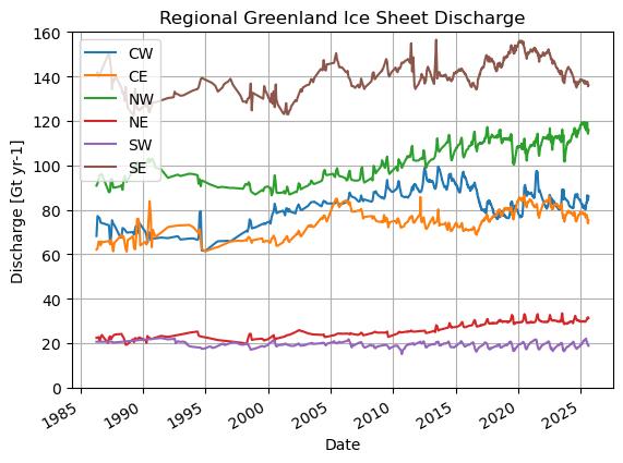
12.2. Region Discharge#
region_d_df = pd.read_csv(links['region_D.csv'], parse_dates=['Date'])
region_d_df
| Date | CE | CW | NE | NO | NW | SE | SW | |
|---|---|---|---|---|---|---|---|---|
| 0 | 1986-04-15 | 62.137103 | 68.260368 | 22.420875 | 21.088441 | 90.888020 | 141.065906 | 20.667821 |
| 1 | 1986-05-15 | 62.681844 | 77.211197 | 22.551619 | 20.375301 | 91.876267 | 141.948529 | 20.667821 |
| 2 | 1986-06-15 | 65.678520 | 76.699118 | 22.784760 | 23.760039 | 93.772264 | 139.823480 | 20.667821 |
| 3 | 1986-07-15 | 65.633344 | 76.246051 | 20.908024 | 24.905824 | 95.793717 | 140.318272 | 20.667821 |
| 4 | 1986-08-15 | 64.001971 | 74.264191 | 22.652118 | 23.707009 | 95.469182 | 141.839283 | 20.667821 |
| ... | ... | ... | ... | ... | ... | ... | ... | ... |
| 2920 | 2025-07-03 | 77.428632 | 83.229713 | 30.684348 | 27.458049 | 117.777602 | 137.209408 | 20.424536 |
| 2921 | 2025-07-15 | 76.549233 | 86.581371 | 31.374898 | 28.080070 | 119.337322 | 137.679265 | 20.274452 |
| 2922 | 2025-07-27 | 74.588720 | 85.175539 | 31.497871 | 28.159406 | 114.859978 | 137.485715 | 19.457482 |
| 2923 | 2025-08-08 | 73.874844 | 84.292667 | 31.709303 | 28.196223 | 114.246686 | 135.567358 | 18.872074 |
| 2924 | 2025-08-20 | 75.351757 | 86.121670 | 31.249736 | 28.125413 | 115.976991 | 136.081063 | 18.862323 |
2925 rows × 8 columns
fig, ax = plt.subplots()

ax = region_d_df.plot(x='Date', y=['CW','CE','NW','NE','SW','SE'], ax=ax)

ax.grid()
ax.set_ylabel('Discharge [Gt yr-1]')
ax.set_ylim(0, 160)
ax.set_title('Regional Greenland Ice Sheet Discharge')
Text(0.5, 1.0, 'Regional Greenland Ice Sheet Discharge')
12.3. Specific Basins#
Divided into basins from Mouginot and Rignot (2019).
sector_d_df = pd.read_csv(links['sector_D.csv'], parse_dates=['Date'])
sector_err_df = pd.read_csv(links['sector_err.csv'], parse_dates=['Date'])
We can see what basin names are available by printing the columns (or, in practice, probably by consulting the Mouginot and Rignot vector dataset in GIS software). I will leave this commented out for now so as now to produce a wall of text.
# for c in sector_d_df.columns:
#     print(c)
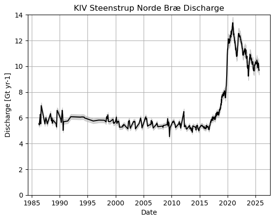
Let’s get an example glaciers - KIV Steenstrup Norde Bræ (I have a vested interest).
# KIV_STEENSTRUP_NODRE_BRAE
kiv_d_df = sector_d_df[['Date', 'KIV_STEENSTRUP_NODRE_BRAE']].rename(columns={"KIV_STEENSTRUP_NODRE_BRAE": "Discharge [Gt yr-1]"})
kiv_err_df = sector_err_df[['Date', 'KIV_STEENSTRUP_NODRE_BRAE']].rename(columns={"KIV_STEENSTRUP_NODRE_BRAE": "Discharge Error [Gt yr-1]"})
kiv_df = pd.merge(kiv_d_df, kiv_err_df, on='Date', how='inner')
kiv_df
| Date | Discharge [Gt yr-1] | Discharge Error [Gt yr-1] | |
|---|---|---|---|
| 0 | 1986-04-15 | 5.528626 | 0.172375 |
| 1 | 1986-05-15 | 5.442344 | 0.169099 |
| 2 | 1986-06-15 | 5.883271 | 0.197025 |
| 3 | 1986-07-15 | 6.258195 | 0.204638 |
| 4 | 1986-08-15 | 5.526404 | 0.176612 |
| ... | ... | ... | ... |
| 2920 | 2025-07-03 | 10.241080 | 0.364027 |
| 2921 | 2025-07-15 | 10.143594 | 0.358980 |
| 2922 | 2025-07-27 | 9.781145 | 0.348199 |
| 2923 | 2025-08-08 | 9.675594 | 0.343677 |
| 2924 | 2025-08-20 | 9.700606 | 0.343281 |
2925 rows × 3 columns
fig, ax = plt.subplots()

ax.plot(kiv_df['Date'], kiv_df['Discharge [Gt yr-1]'], color='black')
ax.fill_between(
    kiv_df['Date'],
    kiv_df['Discharge [Gt yr-1]'] - kiv_df['Discharge Error [Gt yr-1]'],
    kiv_df['Discharge [Gt yr-1]'] + kiv_df['Discharge Error [Gt yr-1]'],
    color='grey', alpha=0.3
)

ax.grid()
ax.set_ylim(0, 14)
ax.set_xlabel('Date')
ax.set_ylabel('Discharge [Gt yr-1]')
ax.set_title('KIV Steenstrup Norde Bræ Discharge')
Text(0.5, 1.0, 'KIV Steenstrup Norde Bræ Discharge')